Kinetic Biochemistry
Lorentz JÄNTSCHI
Technical University of Cluj-Napoca, Romania, http://lori.academicdirect.ro
Abstract: Mathematics and computer programming have a major contribution to chemistry. Two directions can be identified: one that searches and tries (rich) to explain the structural binding and shape of the chemical compounds [1] with major applications in QSPR/QSAR studies [2], and applied sciences such as engineering of materials or agriculture [3]; the second direction is to models the kinetic processes that are involved in chemical reactions [4]. Many such models are available here. The present paper describes three variants of well the known kinetic models and presents the mathematical equations associated with them. The differential equations are numerically solved and fitted with MathCad program.
Keywords: numerical methods, kinetics, oscillating reactions
Introduction
The oscillating reactions are the most spectacular and essential for life [5]. All live processes are based on one or more oscillating reactions [6,7].
The possibility of periodically altering the concentrations of the reactants, the agents and the product, in space and time, is a result of the autocatalysis. Fig. 1 represents two temporary aspects of the space distribution (distribution in space) of the reaction products through the concentration wave front in the proximity of the electron participates in the reaction as a reactant.
The oscillating reactions are more than a laboratory curiosity [8,9]. If in the industrial processes they appear in few cases, in biochemical systems there are numerous examples of oscillating reactions [10,11]. For instance, the oscillating reactions maintain the rhythm [12,13].

Fig. 1. Concentration gradient in an oscillating reaction at the t, and at the t + ∆t moments;
Avi animation: http://lori.academicdirect.ro/free/RO.avi
A general characteristic of the oscillating reactions in that, under the same conditions, all the participants from the reaction chain oscillate with the same frequency but a different displacement (lagging) shift.
1. Diffusion
In case of liquid phase, reactant particles must pass through solvent particles and collisions of reactants are not frequent such in gases, the mobility of them is much lower [14]. From this reason, the collision time is bigger and in this time interval of molecules contact appear the probability that the system of molecules to accumulate enough energy to react. The molecules of reactant are permanently surrounded by solvent molecules and must be considered the entire energy of local assembly. More, the molecules of solvent can active participate to reaction as intermediary catalyst of process [15, 16]. In conclusion, the global reaction process in liquids is more complex then gases [17, 18]. Anyway, it can be decomposed in simple processes through establishing of a kinetic scheme [19,20].
Let a reaction through two reactants, R1 and R2 and let κd be the forming constant of R1R2 compound. The reaction process is expressed by:
![]() , ν = κd∙[R1]∙[R2] (1)
, ν = κd∙[R1]∙[R2] (1)
Forming of R1R2 is determined by diffusion characteristics of R1 and R2. Assuming that the reaction (1) has a spherical symmetry, the diffusion equation of property à in space (r) and time (t) are expressed by:
![]() (2)
(2)
If R2 diffuses through R1, then R1 are in the center of coordinate reference and if diffusing property à is R2 concentration [R2], then (2) become:
![]() (3)
(3)
Reducing the diffusion process to the stationary case, (3) are annulling:
![]() (4)
(4)
To solve and fit the concentration gradient of R2 a second order differential equation must be solved:
![]() (5)
(5)
The equation (5) has two constants after integration, which it result from limit conditions. For simplifying, let us note:
![]() (6)
(6)
With (6), the equation (5) becomes:
![]() (7)
(7)
By multiplying of (7) with dr/r2, it becomes a simple differential equation:
![]() (8)
(8)
The equation (8) can be integrated member by member, when it results:
![]() (9)
(9)
where a is a integration constant. Using again (6) the resulted equation (9) becomes:
![]() (10)
(10)
By integration of (10), it result expression of [R2] depending on radius r:
![]() (11)
(11)
The value of a, and b parameters are determined from:
b = [R2](∞) = [R2]∞ and [R2](r0) = 0 (12)
where first equality express the fact that at huge distance from R1 molecules, where R2 concentration is observed one from mass of solution, [R2]0, and the second equality express the fact that there exist r0 coordinate from R1 molecules where concentration of R2 are null through reaction of R1 and R2. More, r0 is the coordinate at which molecules are close enough to react. The reaction is not instant, such as we can believe. This phenomenon is explained by fact that the relation (11) does not contain the temporal coordinate, t.
Expressing the relations (11) and (12) through the entire space (r>0) we obtain:
 (13)
(13)
equation that are fitted in following graph:
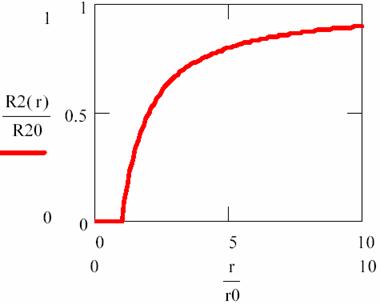
Fig. 2. Variation of R2 in vicinity of R1 molecules (diffusion and reaction phenomena)
The radial flux of [R2] is:
 (14)
(14)
and at coordinate of reaction the radial flux is:
![]() (15)
(15)
The mean value of concentration that crosses the surface 4·π·r02 in a one unit of time (the variation of concentration in time, rate of concentration variation through surface) is:
![]() (16)
(16)
Reaction rate of R2 with molecules of R1, noted with u21 are obtained multiplying this quantity (expressed by 16) with number of R1 molecules from one unity of volume (with [R1]0·NA):
u21 = -4πr0![]() [R2]∞[R1]∞NA (17)
[R2]∞[R1]∞NA (17)
Repeating these calculations for hypothesis of R1 molecules diffusion through field of R2 molecules, it results:
u12 = -4πr0![]() [R2]∞[R1]∞NA (18)
[R2]∞[R1]∞NA (18)
Real rate of reaction u are a mean value of these theoretical results obtained through model simplifying in hypothesis that R2 diffuse to R1 and respectively R1 diffuse to R2. In reality, these phenomena are present simultaneously and competitive:
u = (u12 + u21)/2
= -4πr0D[R2]∞[R1]∞NA,
D = (![]() +
+![]() )/2 (19)
)/2 (19)
The minus sign in expression of rate u is because of reference system chousing, the diffusion is from big positive values of r to small positive values of them. The values [R2]∞ and [R1]∞ are concentrations recorded in mass of solution (more exactly [R1] and [R2]) it result the value of rate constant for a reaction controlled by diffusion in spherical symmetry:
κd = 4πr0DNA (20)
The pair R1R2 can also to dissociate through a process without reaction, so:
![]() , u = κd'[R1R2],
κd' = 4πr0'D'NA (21)
, u = κd'[R1R2],
κd' = 4πr0'D'NA (21)
or can form reaction products (different from R1 and R2):
![]() , u = κp[R1R2],
κp = 4πr0''D''NA (22)
, u = κp[R1R2],
κp = 4πr0''D''NA (22)
Let us come back to hypothesis of stationary (time independence). Mass of reaction is constant in most of time, such that the [R1R2] concentration of pairs is ready to consume and to form products or to become again reactants. Expressing this fact, we can write:
![]() (23)
(23)
and, replacing the expressions of ![]() :
:
κd[R1][R2]
= (κd'+κp)∙[R1R2],
![]() (24)
(24)
The equation (22) is only one that contains also the rate of products forming. Using (22) and (24), it results:
uj = βjκp[R1][R2] = ![]() (25)
(25)
The equation (25) has two limit cases. When κd'![]() κp
the equation (25) becomes:
κp
the equation (25) becomes:
uj = βjκp[R1][R2] = βjκd[R1][R2] (26)
and the reaction are controlled in exclusivity by diffusive
capacity of reactants. When κp![]() κd'
the equation (25) becomes:
κd'
the equation (25) becomes:
uj = βjκp[R1][R2] = βj(κdκp/κd')[R1][R2] (27)
where are easy to observe that κd/is equilibrium constant of the reaction:
![]() , Κ = κd/κd' (28)
, Κ = κd/κd' (28)
and in this case the diffusive control disappear (see expressions of κd and κd') and the reaction are controlled kinetically and the transformation into products are make with energy consuming from environment (the energy are accumulate in collision pair from surrounding molecules of solvent).
2. Mass Balance in Controlled by Diffusion Reactions
The general equation of diffusion can be written in Cartesian coordinates:
![]() (x,y,z,t) = ΚΔÃ(x,y,z,t) -
(x,y,z,t) = ΚΔÃ(x,y,z,t) - ![]() (
(![]() +
+![]() +
+![]() )Ã(x,y,z,t)v(x,y,z,t) (29)
)Ã(x,y,z,t)v(x,y,z,t) (29)
where is assumed that diffusion are joined also by convection, which is transport of property makes through solvent movement. The equation (29) are established based on diffusion and convection phenomena in a space region ((x,y,z),(x+dx,y+dy,z+dz)) without considering a possible reaction that can decrease or increase the value of à property in considered space region. A reaction is possible and is generally independent of space coordinates. Expressing his dependence, we can write:
![]() (x,y,z,t) = κ
(x,y,z,t) = κ![]() (30)
(30)
where γà is reaction order. Completing the equation (29) with the term from (30), it results:
![]() (x,y,z,t) = ΚΔÃ(x,y,z,t)-
(x,y,z,t) = ΚΔÃ(x,y,z,t)-![]() (
(![]() +
+![]() +
+![]() )Ã(x,y,z,t)v(x,y,z,t)+κ
)Ã(x,y,z,t)v(x,y,z,t)+κ![]() (31)
(31)
The equation (31) named the equation of mass balance for the property à and is applied in numerous chemical processes. Two such examples are the diffusion of oxygen in blood and the diffusion of a gas to the surface of a catalyst [21, 22]. The solutions of (31) equation are not easy to obtain. The equation is a inhomogeneous differential one. The analytical solving is possible only in few special cases. For projecting of chemical reactors and kinetic biochemistry analysis that use this equation, are makes through numerical methods based on a specific real model of reaction [23].
Expressing the equation (31) in one-dimensional case without convection and with a property consume of 1 reaction order (γà = 1), it result:
![]() (x,t) = Κ
(x,t) = Κ![]() (x,t) + κÃ(x,t) (32)
(x,t) + κÃ(x,t) (32)
If a function Q(x,t) is a solution of equation without reaction, then:
![]() (x,t) = Κ
(x,t) = Κ![]() (x,t) (33)
(x,t) (33)
and Ã(x,t) are given by:
Ã(x,t) = Q(x,t)eκt (34)
is a solution of equation with reaction (equation 32).
About the equation (33) and his solution, it is completely
solved using distribution theory [24]. The general solution of (33) in ![]() space (x = (x1,
..., xn)) is:
space (x = (x1,
..., xn)) is:
 (35)
(35)
For n = 1 (![]() ) we obtain the solution of equation (33).
Replacing in (34) this solution, it results:
) we obtain the solution of equation (33).
Replacing in (34) this solution, it results:
![]() (36)
(36)
Particular solutions of these equations are plotted in figs. 3-5.
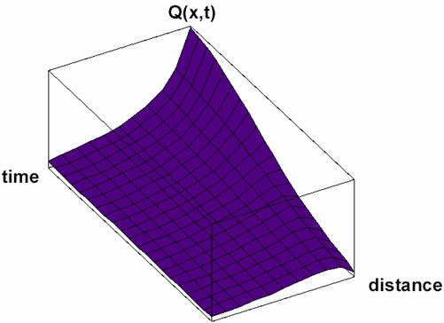
Fig. 3. Space and time dependence of property à with diffusion:
solution Q(x,t) of (33) for Κ = 2
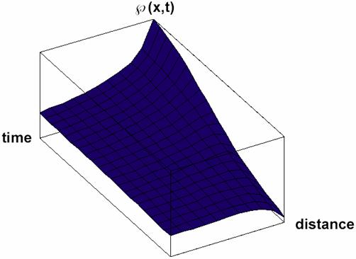
Fig. 4. Space and time dependence of property à with diffusion and property forming
(κ>0 in equation 32) solution Ã(x,t) of (32) for Κ = 2 and κ = 3
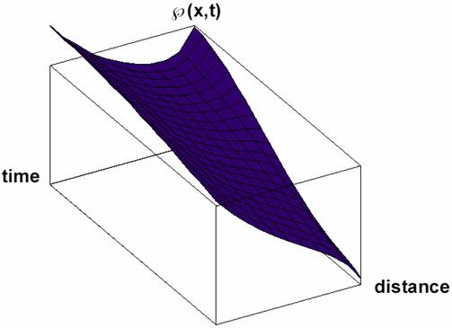
Fig. 5. Space and time dependence of property à with diffusion and property consuming (κ<0 in equation 32) solution Ã(x,t) of (32) for Κ = 2 and κ = -3
3. Monomolecular Reactions
In a monomolecular reaction a single molecule go through a structure rearrangement or decomposition [25]. Such process is rearrangement of cyclopropane to propene:
![]()
The general case of monomolecular reaction is governed by the equation:
R → ΣjβjPj,
j = 1, …, J, ![]() = - κ[R] (37)
= - κ[R] (37)
The rate law for such a reaction is written directly based on chemical equation of reaction. Rearrangement of propene has, according to (37) a single product of reaction, so J = 1 and βJ = 1. A monomolecular reaction is of order 1 because molecules number from reactant which are decomposing in a short time interval are directly proportional with number of molecules available to react, so with [R].
4. Bimolecular Reactions
In such a reaction have collision and exchange energy two molecules, atoms or group of atoms. Note that the implied species can make also other exchanges (such as electrons). Bimolecular reaction is also the equations of following type, between methyl iodide and ethylic alcohol in alcohol medium:
CH3I + CH3CH2O- → CH3CH2OCH3 + I-
The mechanism of this reaction is bimolecular, proved by experimental rate law:
ν = κ[CH3][CH3CH2O]
Generally,
R1 + R2 →
ΣjβjPj, j = 1, …, J, ![]() = - κ[R1][R2] (38)
= - κ[R1][R2] (38)
A bimolecular reaction is of order 2 because his rate is proportionally with speed of reactants in moment of collision, so with his concentrations.
Any assumption related to the mechanism of a reaction, including the reactions of order 2 mechanisms, must be followed by testing phase of assumed model.
Note that the correspondence between order of a reaction and reaction type is not a bi-univocal one. Thus, if reaction is an elementary process of second order, then the order of reaction is two. Reverse, if order of reaction is two, reaction may be following a complex mechanism. The postulated mechanism can be augmented through investigation of secondary products and intermediaries.
5. Monomolecular Consecutive Reactions
Another elementary case is for monomolecular consecutive reactions [26,27], such as radioactive fission [28,29]:
239U → 239Np → 239Pu, T1/2(239U, 239Np) = 23.5 minutes; T1/2(239U, 239Pu) = 2.35 days;
R1 → R2 → … → Rn (39)
Let κ1,2, ..., κn-1,n be the rate constants of monomolecular processes Ri → Ri+1. Then, the decomposition rate of R1 is given by:
![]() = - κ1,2[R1] (40)
= - κ1,2[R1] (40)
and global rates of R2, …, Rn-1 intermediaries forming are given by the differences between rate of his forming reaction and rate of his decomposing reaction [30]:
![]() = - κj,j+1[Rj]
+ κj-1,j[Rj-1], j = 2, …, n-1 (41)
= - κj,j+1[Rj]
+ κj-1,j[Rj-1], j = 2, …, n-1 (41)
Forming rate of final product Rn is given by an expression similarly to (40):
![]() = κn-1,n[Rn-1] (42)
= κn-1,n[Rn-1] (42)
Integration of (40) lead to:
[R1] = [R1]0![]() (43)
(43)
If are assumed that initially only R1 are present ([Rj]0 = 0, j > 1), then the (41) equations solutions can be obtained successively and the first integration lead to:
![]() (44)
(44)
Is complicate to go on with formal solving of differential equations system (41), replacing of (44) in (41) conduct us at inhomogeneous differential equation of order 1, but can be solved elegantly using a formal or numeric specialized software. The identifying of the integration constants that appear at solving steps is makes with respect to initial values of concentrations (in our case [Rj]0 = 0 for j > 0) and the equation of concentration balance:
[R1] + [R2] + … + [Rn] = [R1]0 + [R2]0 + … + [Rn]0 (45)
In particular case taken from literature [31] of n = 3 and [R2]0 = [R3]0 = 0, the expression of [R3] is:
 (46)
(46)
and in figure 6, are depicted the dependencies in this particular case.
The point of maximum for R2 concentration is obtaining from annulling first order derivate of concentration:
 (47)
(47)
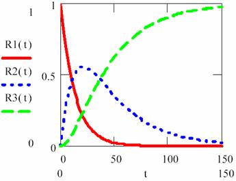
Fig. 6. Concentrations variations for three consecutive monomolecular reactions
with [R1]0 = 1 mol·l-1, [R2]0 = [R3]0 = 0 mol·l-1, κ1,2 = 3/40, κ2,3= 2/71
The equations system:
 (48)
(48)
are very useful in practice, when are measured the time t2,max and the concentration [R2]max and after that are identified the values of rate constants κ1,2 and κ2,3.
If we start from (46) with substitution Κ = κ2,3/κ1,2 and proper grouping of terms it result:
 (49)
(49)
The equation (49) expresses a dependency of [R3]/[R1]0 by time and Κ for a choused decomposing reaction R1 > R2 and a 3D dependency was plotted in fig. 7.
For Κ < 1 (κ2,3 < κ1,2) the determining rate stage is first stage (R1 > R2) until the time rich the value of 104 s. In this time interval (0-104 s) with high priority are accumulating the R2 intermediary and after that, in short time, R2 are transformed to R3.
For Κ > 1 (κ2,3 > κ1,2) the determining rate stage is second stage (R2 > R3) it was in fact the responsible for surface shape for lg(κ2,3/κ1,2)+5 > 5.
The figure 7 proves that in a process that evolve through consecutive reactions, for rate constant significant different there exist always a stage that determinate reaction rate, and these is the stage that evolve with lowest rate.
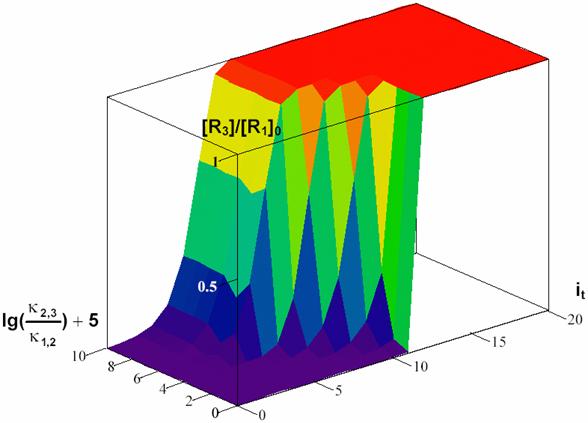
Fig.
7. Surface of R3 forming depending on forming rate (expressed by κ2,3/κ1,2
value) and time (expressed by it value) for κ1,2
= ½ and t = ![]() -1,
it = 0, …, 20, Κ = κ2,3/κ1,2
= 10j-5, j = 0, …, 10
-1,
it = 0, …, 20, Κ = κ2,3/κ1,2
= 10j-5, j = 0, …, 10
6. Pre-equilibrium
The case of chemical reactions that evolve governed by equation:
![]() (50)
(50)
will be discussed in this section.
The equation (50) implies a pre-equilibrium, the state in which a intermediary (R3) are in equilibrium with the reactants [32, 33]. Pre-equilibrium appear practically when the forming rate of intermediary and decomposing rate of them into reactants are much higher then products forming rate [34]:
κ1,
κ2 ![]() κ3 (51)
κ3 (51)
If (51) are true, it can be considered that R1, R2 and R3 are in equilibrium and:
[R3]/([R1][R2]) = κ1/κ2 = Κ (52)
From following equation, the forming rate of R4 can be determined:
![]() = κ3[R3]
= κ3Κ[R1][R2] (53)
= κ3[R3]
= κ3Κ[R1][R2] (53)
The (53) equation type is a second order one with rate constant κ given by:
κ = κ3Κ = κ3κ1/κ2 (54)
If we don’t ignore the fact that R3 > R4 is a slow reaction, we can use the approximation of stationary phase on R3:
![]() = κ1[R1][R2]
- κ2[R3] - κ3[R3] = 0 (55)
= κ1[R1][R2]
- κ2[R3] - κ3[R3] = 0 (55)
and reaction rate will be:
![]() = κ3·[R3]
= κ[R1][R2], κ
=
= κ3·[R3]
= κ[R1][R2], κ
= ![]() (56)
(56)
7. Michaelis – Menten Mechanism
Michaelis – Menten mechanism work with respect to the equation [35]:
![]() (57)
(57)
and are frequently applied at enzymatic catalysis (where R1 are enzyme, R2 are substrate and R3 it cumulate the obtained products after enzyme action [36,37].
The rate of enzymatic catalyzed reaction [38] depends on enzyme concentration [R1] even if the enzyme do not go through a net change (are achieve in reaction products, [39]). If we follow the same judgment of stationary phase (equation 55):
![]() = κ1[R1][R2]
– κ2[R1R2] – κ3[R1R2] (58)
= κ1[R1][R2]
– κ2[R1R2] – κ3[R1R2] (58)
From (58) it result the expression of [R1R2]:
[R1][R2] = ![]() [R1][R2] (59)
[R1][R2] (59)
Concentration balance is:
[R1]0 = [R1] + [R1R2] (60)
If we substitute [R1] from (60) into (59), it results:
[R1R2] = ![]() [R2]([R1]0
– [R1R2]) (61)
[R2]([R1]0
– [R1R2]) (61)
From (61) [R1R2] can be extracted. Then result:
[R1R2] = ![]() [R1]0[R2] (62)
[R1]0[R2] (62)
Forming rate of R3 (like equation 56) is:
![]() = κ3[R1R2]
=
= κ3[R1R2]
=  [R2][R1]0 (63)
The ΚM are named Michaelis constant and are given by:
ΚM
= ![]() (64)
(64)
Using (63) and (64) the general expression of R3 forming rate (hardly used in enzymatic catalysis) is:
![]() = κ[R1]0, κ =
= κ[R1]0, κ = ![]() (65)
(65)
To express the dependency of κ constant by [R2] substrate concentration, the following equation is useful:
κ = ![]() (66)
(66)
κ’s dependency of [R2]/ΚM value are fitted in fig. 8.
Usually, the enzyme quantity is much lower than substrate quantity, so we have:
[R2] ![]() [R1R2],
[R2]
[R1R2],
[R2]![]() [R0] (67)
[R0] (67)
The (67) equation it correspond to horizontal portion of dependency from fig. 8 and describe most of the enzymatic process evolution (until the vicinity of final point). If (67) are replaced in (65), it results:
![]() = κ[R1]0, κ =
= κ[R1]0, κ = ![]() (68)
(68)
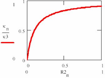
Fig. 8. Rate constant (κ) in Michaelis – Menten mechanism (n are iteration number)
The Michaelis - Menten mechanism are also successfully applied to inorganic reactions [40].
8. Lindemann – Hinshelwood Mechanism
Chemical processes evolve in reality in a much complex mode than can be expressed through the mechanisms presented until now. These are only approximations, and have serious difficulties and limitations when we want a deeper study of reactions mechanism [41,42]. A prove of this fact are the studies initiated by Lindemann and completed by Hinshelwood for case of monomolecular reactions. Them proposed model, that assume that reactant molecule require activation to pass into products are depicted in fig. 9.
The mechanism consists in:
1. collision of two fast molecules R:
R+ R ![]() R* + R,
R* + R, ![]() , * energetic
excited molecule (69)
, * energetic
excited molecule (69)
2. collision of a energetic excited molecule R* with unexcited one:
R* + R![]() R+ R,
R+ R, ![]() (70)
(70)
3. transformation of energetic excited molecule into products:
R* ![]() P,
P, ![]() (71)
(71)
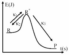
Fig. 9. Energetic activation in Lindemann – Hinshelwood Mechanism
From experimental observations, which show that global reaction has a kinetic of order 1, such as we presented through (37) equation, it result that the main rate phase (slowest one) is third one (κ3 < κ1, κ2). At same result are done if stationary phase approximation for R* is applied:
![]() (72)
(72)
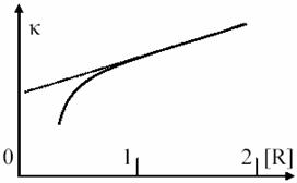
Fig. 10. Linearity approximation in monomolecular processes vs. L–H Mechanism
Rate equation is:
![]() , where
, where ![]() (73)
(73)
At limit, when κ3 << κ2[R] and κ3 are ignored in relation to κ2[R], the (37) equation is obtained, according to the simplified model of monomolecular processes. Dependence of κ constant by reactant concentration is depicted in fig. 10.
The Lindemann – Hinshelwood model are capable to
explain the changing of reaction order for monomolecular reactions when [R]
concentration is lower [43], but does not provide a detailed explanation of
real processes. κ’s dependence curvature is even more significant in reality
for very low concentrations of [R] then predicted curvature from second order
kinetic reaction. An adjusting of this model was makes by Rice, Ramsperger and Kassel
[44], which replace the third stage (R* ![]() P) with:
P) with:
![]() (74)
(74)
where R* is the molecule with high energy and R†
is activated molecule. They introduce a rate constant for every stage. This
construction has explanation that the accumulated energy is distributed to all
bonds from molecule. It result that exist a delay in transition of R* to
products, provoked by previous forming of activated molecule R† (R*
![]() R†).
R†).
Using the differential equation system:
 (75)
(75)
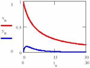
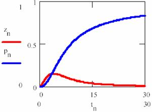
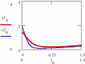
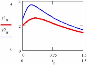
obtained based on equations (69), (70) and (74) a graphical dependences of reactant [R], product [P] and intermediaries [R*], [R+] was plotted in fig. 11 and 12 for rate constants κ1 = 0.2, κ2 = 0.1, κ3 = 0.9 and κ4 = 0.5 with initial concentration of R [R] = x0 = 1 and time interval tn = 0, …, 30.
|
|
|
|
Fig. 11. Concentration – time dependence for reactant R (xn on graph) and R* (yn on graph), eq. 75 |
Fig. 12. Concentration – time dependence for product P (pn on graph) and R+ (zn on graph), eq. 75 |
9. Catalyzed Processes
If activation energy of a reaction is big, only a small ratio of molecular collisions produces reaction. The catalysts has role to decrease the activation energy of the reaction by providing another way to pass to products, that avoid the slow rate stage of reaction and lead to a increased rate of reaction, at same temperature [45,46].
Here an example of catalyzed reaction: activation energy for H2O2 decomposing in solution is 76kJ·mol-1 and the reaction is slow at room temperature. If we add iodine in small quantities, the activation energy decrease at 57 kJ·mol-1 and the reaction rate grows about 2000 times [47].
Enzymes are biological catalyst. It is very specific and can have a spectacular effect on his controlled reactions. The activation energy for acid hydrolysis of sucrose is of 107 kJ·mol-1. In presence of sucrase enzyme, the energy is decreased to 36 kJ·mol-1 and hydrolysis process is accelerated about 1012 times at body temperature (310 K).
A homogenous catalyst is in same phase with reaction mixture. Exist also heterogeneous catalysts (placed somewhere else than reaction mixture) such as a solid catalyst for a gas phase reaction [48,49].
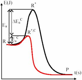
Fig. 13. Energetic tunneling with catalysts
The fig. 13 presents the corridor tunneling from reactants to products by using catalyst. The most important cases of homogenous catalysis are base catalysis and acid catalysis. They are implied frequently organic reactions, each one or both. The easiest action mode of them is through Brönsted mechanism. Therefore, Brönsted acid catalysis consists in a proton transfer to the S substrate from a HA acid:
S + HA ![]() HS+
+ A-, HS+ + R
HS+
+ A-, HS+ + R ![]() Products (76)
Products (76)
This process is primary one in ester solvolysis [50,51] keto-enolic tautomery and sucrose inversion [52,53]. Brönsted base catalysis consists in a proton transfer from S substrate to B base:
SH + B ![]() S-
+ BH+, S-+ R
S-
+ BH+, S-+ R ![]() Products (77)
Products (77)
This process is primary one in isomerisation and halogenation of organic compounds, and at Claisen and aldolyc reactions [54, 55].
Autocatalysis phenomena consists in acceleration of a reaction makes by his products [56, 57]. An example of autocatalysed reaction is:
R ![]() P, with rate
law υ = κ[R][P] (78)
P, with rate
law υ = κ[R][P] (78)
In equation (78) the reaction rate is increased together with reaction products formation. Expressing the variation of product concentration, it results:
![]() (79)
(79)
By integration of the (79) equation we obtain:
![]() (80)
(80)
where C is obtained from initial conditions. Resolving the initial conditions in (80):
![]() (81)
(81)
or:
![]() (82)
(82)
and:
 (83)
(83)
The (83) equation allows us to express the [P] concentration depending only by time and initial conditions:
![]() (84)
(84)
The (84) equation are plotted in fig. 14, for [P]0 = 0.1, [R]0 = 0.99, κ = 4:
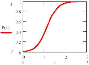
Fig. 14. Variation of product concentration in an autocatalysed reaction
The reaction rate is obtained from (84) equation differentiating or through (84) substitution into (79).
It can be observed that the reaction rate is small at beginning and increase together with P product forming until his maximum value (for [P] = [R]). After that, it has decrease, such as can be observed in fig. 15.
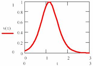
Fig. 15. Product’s concentration variation rate into a autocatalysed reaction
If we are interested to find the time moment when the reaction rate is maximum, the following equation are useful:
 (85)
(85)
The industrial importance of autocatalysis is significant [58]. Therefore, autocatalysis appears in oxidation reactions, when autocatalysis study allow to maximize the reaction rate through continue assuring of optimal concentrations of reactant and product. This is the field of automated industrial processes.
10. Explosions
Rapid increasing of rate constant by temperature provokes a thermo explosion [59,60]. If the reaction is exothermic one, and provoke increasing of reaction environment increasing then acceleration of reaction rate it has as result a much faster increasing of both temperature and reaction rate [61]. To exemplifying, let us assume that temperature is linear increased by products concentration (then decrease proportionally with reactant concentration) and rate constant is increased with temperature through Arrhenius law:
![]() (86)
(86)
If we express the κ constant by [R]:
![]() (87)
(87)
and assume that the reaction is first order one by concentration:
![]() = - κ[R] (88)
= - κ[R] (88)
we can replace the κ value from (87):
![]() = - κ0eαβ[R][R] (89)
= - κ0eαβ[R][R] (89)
Separating now the variables:
0 = κ0eαβ[R][R]-1d[R] + κ0dt (90)
By integration of (90) it results:
 (91)
(91)
which is a t = t([R]) dependency.
By fitting this dependency (fig. 16) and reversing it, the [R] = [R](t) dependency is obtained:
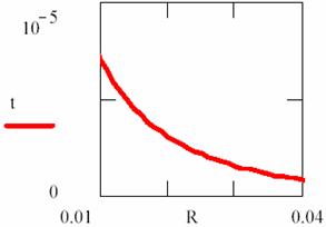
Fig. 16. Explosion phenomena, t = t([R]) diagram
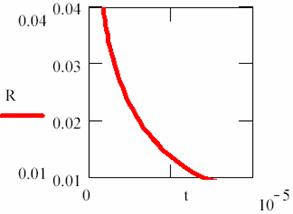
Fig. 17. Explosion phenomena, [R] = [R](t) diagram
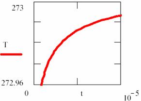
Fig. 18. Explosion phenomena, T = T(t) diagram
Using the (86) relation, we can also plot the T = T(t) dependency (fig. 18). The explosion phenomena are explained by fact that the slope of [R] = [R](t) and T = T(t) curves are vertically in t = 0 (17 and 18 figures). Consuming of most of [R] reactant quantity, such as we can observe on graphs, fitted for α = 1, β = 40, κ = 105, it correspond to a short time.
The final point of explosion has, of course, [R] = [R](t) and T = T(t) null curves slope.
The experimental study of explosion that are produced when oxygen and hydrogen react:
2H2 + O2 → 2H2O (92)
allowing to establish the following mechanism:
 (93)
(93)
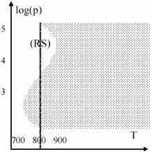
Fig. 19. H2 + O2 explosion
Other secondary reaction was identified, such as:
O=O + ·H → ·O–OH (94)
Such as temperature, also the pressure plays an important role in explosions. The 19 figure present the log(p) – temperature diagram for hydrogen + oxygen mixture. Marked area is the explosion area. The presence of (RS) region is explained by secondary reactions of type (94) facilitating.
11. Lotka – Volterra Autocatalytic Oscillator Model
For the first time Lotka [62] suggested a mechanism of a complex reaction, in homogeneous phase (stage), which shows damped oscillations. Ten years later, in his paper, [63] Lotka modified the mechanism suggested in 1910 in order to generate undamped oscillations.
The mechanism is named Lotka-Volterra and it is further presented. The following pattern of reactions is considered:
 (95)
(95)
The last equation (95d), represents an extraction process of the reaction product P, while the stages (95a) and (95b) are autocatalytic. In L-V model of the reaction mechanism, concentration of the reactant R is maintained constant, (for example either by an addition in the reaction vessel or by an equilibrium between two non-miscible phases when necessary). These restrictions cause the concentrations of X and Y intermediaries/agents to be variable / changeable / unsteady:
![]() = υ(29a) – υ(29b) = κ1[R][X] – κ2[X][Y] (96)
= υ(29a) – υ(29b) = κ1[R][X] – κ2[X][Y] (96)
![]() =
υ(29b) – υ(29c) = κ2[X][Y] – κ3[Y] (97)
=
υ(29b) – υ(29c) = κ2[X][Y] – κ3[Y] (97)
(96) and (97) equations form a system of differential equations with the functions [X] = [X](t) and [Y] = [Y](t). This system can be simply solved by a numerical method [64]. Thus, the equations (96) and (97) became:
xn+1 = xn+(tn+1-tn)xn(κ1[R]-κ2yn) (98)
yn+1 = yn+(tn+1-tn)yn(κ2xn-κ3) (99)
With numerical values:
x0 = [X0] = 1, y0 = [Y0] = 1, κ1 = 3, κ2 = 4, κ3 = 5, [R] = 2 (100)
there can be produced/generated the numerical series/systems (xn)n≥0 and (yn)n≥0 corresponding to the temporal series (tn)n≥0.
In order to obtain an as faithful representation of the mechanism as possible a very fine/careful division of the temporal coordinate in the numerical simulation is required.
Thus, considering the series tn = n/105 with n = 0,1,...5·105 there are obtained the representations from figs. 20 and 21 for the concentration of the intermediaries [X] = (xn)n≥0 and [Y] = (yn)n≥0. In the fig. 22 the concentration of the reaction product [P] develops/grows in the time through Pn (the equations 95c and 95d, taking κ4 = 3).
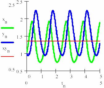
Fig. 20. The oscillation of the intermediaries in L-V mechanism
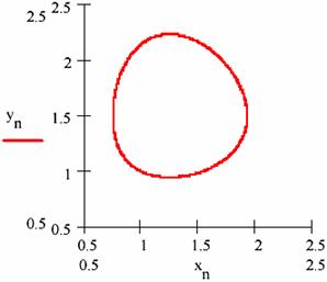
Fig. 21. The variation path ([X],[Y]) in L-V mechanism
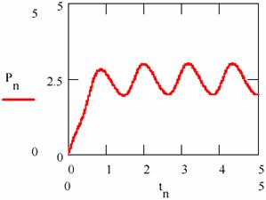
Fig. 22. The variation of the product concentration and storage in L-V mechanism
Carrying out/performing the regression resulted from the equation (95c) and represented in fig. 23, by pn, according to the concentration [P] and depending on time, the regression slope gives the average rate of formation equal to 1.481.
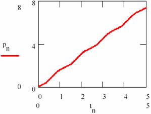
Fig. 23. The variation of the product concentration and storage in L-V mechanism
There are a few remarks to be made, namely: the sum of average concentrations of the agents is maintained in time as the regression equation xyn also is shows (the slope of the regression equation is null). This average sum M([X]) + M([Y]) = 1.365; hence it results that the average concentrations of the agents also remain constant in time; the values of the average concentrations are M([Y]) = 1.468 and M([Y]) = 1.263.
12. A Model of Damped Oscillations
Let it be a chemical process that takes place according to the following model of a reaction mechanism:
 (101)
(101)
As in Lotka – Volterra, model, the concentrations of the R1 and R2 reacting substances remain constant during the process. The solving of the model begins by writing the variation equation for the intermediaries:
![]() = υ(34a)
- 2υ(34b) - υ(34c) = κ1[R1]
- 2κ2[X]2[Y] - κ3[R2][X] (102)
= υ(34a)
- 2υ(34b) - υ(34c) = κ1[R1]
- 2κ2[X]2[Y] - κ3[R2][X] (102)
![]() =
2υ(34b) + υ(34c) - υ(34d) =
2κ2[X]2[Y] + κ3[R2][X] -
κ4[Y] (103)
=
2υ(34b) + υ(34c) - υ(34d) =
2κ2[X]2[Y] + κ3[R2][X] -
κ4[Y] (103)
The equations (102) and (103) form a system of differential equations having the functions [X] = [X](t) and [Y] = [Y](t). This system may also be easily solved by a numerical method. The equations (102, 103) are written thus:
xn+1 = xn + (tn+1 -tn)(κ1[R1] - xn(2κ2xnyn + κ3[R2])) (104)
yn+1 = yn+(tn+1 – tn)(xn(2κ2xnyn + κ3[R2]) - κ4yn) (105)
Having the numerical value:
x0 = 0, y0 = 1, κ1 = 3, κ2 = 4, κ3 = 5, κ4 = 7, [R1] = 2, [R2] = 2 (106)
there can be generated the numerical series (xn)n≥0 and (yn)n≥0 corresponding to the temporal series (tn)n≥0.
Taking into account the series tn = n/100000 with n = 0,1..300000 there are obtained the representation from figs. 24 and 25 for the concentrations of the intermediaries [X] = (xn)n≥0 and [Y] = (yn)n≥0.
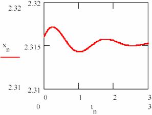
Fig. 24. The damped oscillations in chemical reactions:
the concentration of the intermediary X
Fig. 25 shows that the system tends towards a state of equilibrium state characterized a ratio of the concentrations of the two intermediaries. The system of the agents practically causes damped oscillations around of the equilibrium ratio for two intermediaries. The chart representing the agent concentration [Y] depending on the agent concentration [X] from fig. 26 shows the same thing.
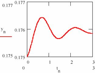
Fig. 25. The damped oscillations in chemical reactions:
the concentration of the intermediary Y
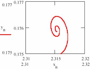
Fig. 26. The damped oscillation path ([X],[Y])
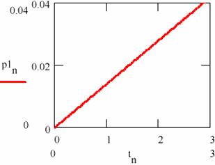
Fig. 27. The linear variation of the amount of products in damped oscillating reactions
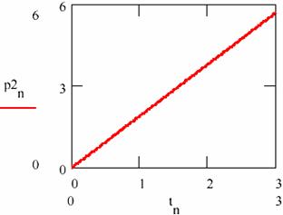
Fig. 28. The linear variation of the amount of products in damped oscillating reactions
The values obtained for the equilibrium concentration are [X] = 2.315 and [Y] = 0.176 and the equilibrium ratio are [X]/[Y] = 13.53.
The dependence on time (tn)n≥0 of the accumulation of the reaction products [P1] = (p1n)n≥0 and [P2] = (p2n)n≥0 is given in figs. 27 and 28.
Figs. 27 and 28 shows that this time the concentration of the reaction products changes linearity even if the concentrations of the agents X and Y oscillate towards the equilibrium value.
13. The Brussel Model of Autocatalytic Oscillation
The brussel model was initiated by a group from Bruxelles directed by Ilya Prigogine it introduce for the first time, mechanism of a reaction whose scheme of evolution converged on an attractor [65].
More authors have changed this variant and have studied the systems running according to this mechanism [66, 67]. Further, a simplified variant is presented:
R → X, υ = κ1[R] (a)
X + 2Y → 3Y, υ = κ2[X][Y]2 (b) (107)
Y → P, υ = κ3·[Y] (c)
As in the previous situations, it is supposed that the concentration of the reacting substance R remains constant and the product P may be extracted from the system by a reaction of the type (101d).
X and Y are the intermediaries again. Their rate equations written based on the mechanism (107) are:
![]() = υ(39a)
- υ(39b) = κ1[R1] - κ2[X][Y]2 (108)
= υ(39a)
- υ(39b) = κ1[R1] - κ2[X][Y]2 (108)
![]() = υ(39b) -
υ(39c) = κ2[X][Y]2 - κ3[Y] (109)
= υ(39b) -
υ(39c) = κ2[X][Y]2 - κ3[Y] (109)
Though the equations (108) and (109) seem simpler, at first sight, they are even more difficult to be solved by integration than (96-97) or (102-103). Moreover, the literature has not recorded their integration into the general case described by (108-109).
Besides, the equations (108-109) do not lead to an attractor model not matter by values of the constants of rate and of the concentrations [R], [X]0 and [Y]0. The attempt of solving (108-109) is full of surprises. For most of the values, a system that develops towards a position of equilibrium is obtained; there are values for which damped oscillations to equilibrium are found again; the un-damped periodical oscillations have also an important role, which is confirmed by the majority of the organisms in which the cellular biochemical processes are based on such oscillations.
The processes taking place within the heart are a conclusive example; the periodical heart beats are due to processes of this type. The importance of these processes is great. This was the reason for which Ilya Prigogine was awarded the Nobel Prize for chemistry in 1977, namely for his theories on the dissipative systems.
The equations (108-109) are simplified [68] if [R] = 1, κ1 = 1 and κ3 = 1, are chosen and when the differential system of equations becomes:
![]() = 1 – κ2xy2;
= 1 – κ2xy2;
![]() = κ2xy2 – y (110)
= κ2xy2 – y (110)
where the derivate related to the time of the x variable was. This system of the differential equation (110) does not offer more chances for an exact resolution either. However, the numerical simulation is made in the same way. Thus, the iteration equation of variation for (110) is written:
xn+1 = xn+(tn+1-tn)(1-κ2xnyn2); yn+1 = yn + (tn+1 - tn)(κ2xnyn2 -yn) (111)
Now let us chouse κ2 = 0.88. Taking into consideration two cases, the first one in which the initial concentrations of the agents are x10 = [X]1,0 = 1.5 and y10 = [Y]1,0 = 2 and second one with x20 = [X]2,0 = 2 and y20 = [Y]2,0 = 2.5. Using the series tn = n/100 with n = 0, 1,…, 150 following representations for the concentrations of the agents [X] = (xn)n≥0 and [Y] = (yn)n≥0 are obtained (figures 29 and 30).
|
|
|
|
Fig. 29. The concentrations of the X intermediaries up to the attractor for two cases with different initial conditions |
Fig. 30. The concentrations of the Y intermediaries up to the attractor for two cases with different initial conditions |
The variation diagram of [Y] depending on [X] and the variation in time of the storage of reaction product are depicted in figure 32.
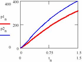
Fig. 31. The product-time dependence in two cases having different initial conditions
Fig. 32. The ([Y], [X]) hodograph two for cases having different initial conditions
An important observation is that the entrance of [Y] related to [X] on the same gravitational orbit for both cases.
If the figures 29 and 30 are not very conclusive and figure 31 seems to confirm this, fig. 32 shows that, though the two systems start from different values of the concentrations of the agents, in both cases the system comes to evolve rather early on the same trajectory.
Now, increasing the time interval by choosing another n = 0,1..3000 the following concentrations of the agents are obtained [X]1 = (x1n)n≥0, [X]2 = (x2n)n≥0, [Y]1 = (y1n)n≥0 and [Y]2 = (y2n)n≥0 for the two cases 1 and 2 of the chosen system (figures 33 and 34). It is noticed that, even if they do not evolve according the same values, same period and amplitude of the oscillations are recorded.
Fig. 33. The periodical evolution having the same different initial conditions
(oscillation period T = 0.226 of [X] and [Y])
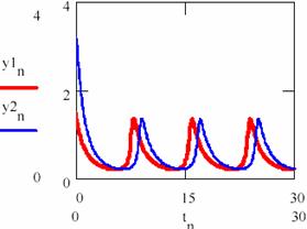
Fig. 34. The periodical evolution having the same different initial conditions
(oscillation period T = 0.226 of [X] and [Y])
Fig. 35 gives the dependence of [Y] under [X] for the cases as well as the accumulation of the product.
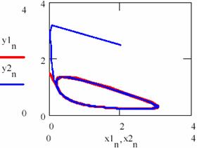
Fig. 35. Convergence at atractor of brusselator system independent from initial conditions
The difference between the Lotka-Voltera model and Bruxelles model one is the following: The Lotka-Voltera model oscillates around the initial values of the concentrations of the agents, whereas the Bruxelles one converges, in time on the same variation equation irrespective of the initial values of the concentrations of the agents. In fact the attractor does not appear for any of their values; for a given k2 there are minimum y0,min and x0,min values from which the periodical oscillations arise and the system tends towards the curve given in fig. 36.
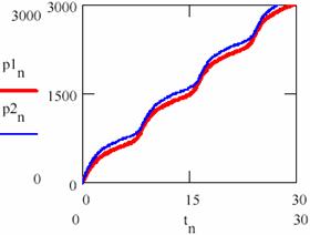
Fig. 36. Different quantities of resulted product for brusselator system
The convergence on the attractor of the brusselator system (a) independent of the initial conditions and (b) different quantities of the product obtained.
Conclusions
There exist a many models of biochemical processes reactions, and every process has some characteristics, as we described below. The importance of every mechanism is given by his applications. It exist much more kinetic models, unexplained in this paper, such as oregonator model [7], one of them implying tens of substances and reactions [69].
As we mentioned before, most spectacular and also important because is most frequent in nature is the brusselator model, every alive organism has one.
The symbolic calculations of reaction rate for biochemical processes are, in most of cases, impossible. In opposite, the numerical modeling of biochemical kinetics proves that it is a very good instrument for mechanism understanding, comparative studies and model validation.
References
1. Diudea M., Gutman I., Jäntschi L., Molecular Topology, Nova Science, Huntington, New York, 332 p., 2001.
2. Diudea M. V., Ed., QSPR / QSAR Studies by Molecular Descriptors, Nova Science, Huntington, New York, 438 p., 2001.
3. Jäntschi L., Microbiology and Toxicology. Phytochemistry Studies (in Romanian), Amici, Cluj-Napoca, 184 p., 2003.
4. Jäntschi L., Unguresan M., Physical Chemistry. Molecular Kinetic and Dynamic (in Romanian), Mediamira, Cluj-Napoca, 159 p., 2001.
5. Jinzhang Gao, Hua Yang, Xiuhui Liu, Jie Ren, Qizhi Li and Jingwan Kang, Determination of glutamic acid by an oscillating chemical reaction using the analyte pulse perturbation technique, Talanta, (6)57, p. 105-114, 2002.
6. Benini O., Cervellati R., and Fetto P., The BZ reaction: experimental and model studies in the physical chemistry laboratory, Journal of Chemical Education, 73, p. 865–868, 1996.
7. Field R.J., Körös E., and Noyes R.M., Oscillations in chemical systems, Part 2. Thorough analysis of temporal oscillations in the bromate-ceriummalonic acid system, Journal of the American Chemical Society, 94, p. 8649–8664, 1972.
8. Field R.J. and Schneider F.W., Oscillating chemical reactions and nonlinear dynamics, Journal of Chemical Education, 66, p. 195–204, 1989.
9. Fitzhugh R., Impulses and physiological states in theoretical models of nerve membrane, Biophysical Journal, 1, p. 445–466, 1961.
10. Gray P. and Scott S.K., Chemical Oscillations and Instabilities: Nonlinear Chemical Kinetics, Oxford Science Publications, Oxford, 1990.
11. Ceroni P., Conti F., Corvaja C., Maggini M., Paolucci F., Roffia S., Scorrano G., and Toffoletti A., Tempo-C61: An Unusual Example of Fulleroid to Methanofullerene Conversion, The Journal of Physical Chemistry A, (1)104, p. 156-163, 2000.
12. Hodgkin A.L. and Huxley A.F., A quantitative description of membrane current and its application to conduction and excitation in nerve, Journal of Physiology, 117, p. 500–544, 1952.
13. Groot J. H. and Brand R., A three-dimensional regression model of the shoulder rhythm, Clinical Biomechanics, (9)16, p. 735-743, 2001.
14. Vanag V.K. and Epstein I.R., Inwardly rotating spiral waves in a reaction diffusion system, Chemical and Engineering News, 79, p. 835–837, 2001.
15. Il-Hie Lee and Ung-In Cho, Pattern Formations with Turing and Hopf Oscillating Pattern in a Discrete Reaction-Diffusion System, Bull. Korean Chem. Soc., (12)21, p. 1213-1216, 2000.
16. Flammersheim H. J. and Opfermann J., Formal kinetic evaluation of reactions with partial diffusion control, Thermochimica Acta, (1-2)337, p. 141-148, 1999.
17. Bartelt-Hunt S. L. and Smith J. A., Measurement of effective air diffusion coefficients for trichloroethene in undisturbed soil cores,Journal of Contaminant Hydrology, (3-4)56, p. 193-208, 2002.
18. Shih-Chin Chang, Ping-Hong Lai, Wei-Liang Chen, Hsu-Huei Weng, Jih-Tsun Ho, Jyh-Seng Wang, Chuan-Yu Chang, Huay-Ben Pan and Chien-Fang Yang, Diffusion-weighted MRI features of brain abscess and cystic or necrotic brain tumors; Comparison with conventional MRI, Clinical Imaging, (4)26, p. 227-236, 2002.
19. Martiel J.-L. and Golbeter A., A model based on receptor desensitization for cyclic AMP signaling in Dictyostelium cells, Biophysical Journal, 52, p. 807–828, 1987.
20. Simon A. M., Doran P. and Paterson R., Assessment of diffusion coupling effects in membrane separation. Part I. Network thermodynamics modelling,Journal of Membrane Science, (2)109, p. 231-246, 1996.
21. Azevedo I. C. A., Oliveira F. A. R. and Drumond M. C., A study on the accuracy and precision of external mass transfer and diffusion coefficients jointly estimated from pseudo-experimental simulated data, Mathematics and Computers in Simulation, (1)48, p. 11-22, 1998.
22. Dou Yi, Maillett H. D., Eich R. F. and Olson J. S., Myoglobin as a model system for designing heme protein based blood substitutes; Biophysical Chemistry, (1-2)98, p. 127-148, 2002.
23. Allegrini P., Benci V., Grigolini P., Hamilton P., Ignaccolo M., Menconi G., Palatella L., Raffaelli G., Scafetta N., Virgilio M. and Yang J., Compression and diffusion: a joint approach to detect complexity, Chaos, Solitons & Fractals, (3)15, p. 517-535, 2003.
24. Trif D., Partial Derivate Equations (in Romanian), for IIIrd year of Informatics, Litho. “Babeş-Bolyai” University of Cluj-Napoca, Faculty of Mathematics, Cluj-Napoca, 1993.
25. Jazbec M., Fletcher D. F. and Haynes B. S., Simulation of the ignition of lean methane mixtures using CFD modelling and a reduced chemistry mechanism, Applied Mathematical Modelling, (8-9)24, p. 689-696, 2000.
26. Ball David W., Kinetics of Consecutive Reactions: First Reaction, First-Order; Second Reaction, Zero Order, J. Chem. Educ., 75, p. 917-918, 1998.
27. Liao W.-H., Chou J.-H. and Horng I.-R., Robust observer-based frequency-shaping optimal vibration control of uncertain flexible linkage mechanisms, Applied Mathematical Modelling, (11)25, p. 923-936, 2001.
28. Kay G., Bateman Equations Simplified for Computer Usage, J. Chem. Educ., 65, p. 970-973, 1988.
29. Pietruszka A. J., Carlson R. W. and Hauri E. H., Precise and accurate measurement of 226Ra-230Th-238U disequilibria in volcanic rocks using plasma ionization multi-collector mass spectrometry, Chemical Geology, (3-4)188, p. 171-191, 2002.
30. Benson S.W., Kinetics of Consecutive Reactions, J. Chem. Phys., 20, p. 1605, 1952.
31. Lysenko A. P., Plyrusnin V. G., Zhur. Fiz. Khim, 32, p. 1074, 1958.
32. Marasinghe P. A. B., Wirth, L. M., A graphical solution of the second-reaction rate constant of a two-step consecutive first-order reaction, J. Chem. Educ., 69, p. 285, 1992.
33. David L. Zechel and Stephen G. Withers, Glycosidase Mechanisms: Anatomy of a Finely Tuned Catalyst, Accounts of Chemical Research; (1)33, p. 11-18, 2000.
34. McLennan A. R., Bryant G. W., Stanmore B. R., and Wall T. F., Ash Formation Mechanisms during pf Combustion in Reducing Conditions, Energy & Fuels; (1)14, p. 150-159, 2000.
35. Michaelis L., Menten M. L., Biochem. Z., 49, p. 333, 1913.
36. Godfrey K. R., Fitch W. R., The deterministic identifiability on nonlinear pharmacokinetic models, Pharmacokinetics and Biopharmaceutics, 12, p. 177-191, 1984.
37. Currie D. J., Estimating Michaelis-Menten parameters: bias variance and experimental design, Biometrics, 38, p. 907-919, 1982.
38. Laidler K. J., The Chemical Kinetics of Enzyme Action, Claredon Press, London, 1958.
39. Ruppert D., Cressie N. and Carroll R. J., A transformation/weighting model for estimating Michaelis-Menten parameters, Biometrics, 45, 637-656, 1989.
40. Grozdanov I., Barlingag C.K., Dey S.K., Ristov M., Najdovski M., Experimental Study of Copper Thiosulfate Systems with Respect to Thin Film Deposition, Thin Solid Films, 250, p. 67-71, 1994.
41. Allpress J. D. and Gowland P. C., Dehalogenases: environmental defence mechanism and model of enzyme evolution, Biochemical Education, (4)26, p. 267-276, 1998.
42. Okano T., Yamada N., Okuhara M., Sakai H. and Sakurai Y., Mechanism of cell detachment from temperature-modulated, hydrophilic-hydrophobic polymer surfaces, Biomaterials, (4)16, p. 297-303, 1995.
43. Glasser L., Rates of bimolecular heterogeneous reactions following the Langmuir-Hinshelwood mechanism, J. Chem. Educ., 56, p. 22, 1979.
44. Cid R., Atanasova P., López Cordero R., Palacios J. M., López Agudo A., Gas Oil Hydrodesulfurization and Pyridine Hydrodenitrogenation over NaY-Supported Nickel Sulfide Catalysts: Effect of NiLoading and Preparation Method, Journal of Catalysis, (2)182, p. 328-338, 1999.
45. Oyama S. Ted, Somorjai Gabor A., Homogeneous, heterogeneous, and enzymatic catalysis, J. Chem. Educ., 65, p. 765, 1988.
46. Lyne P. D. and Karplus M., Determination of the pKa of the 2'-Hydroxyl Group of a Phosphorylated Ribose: Implications for the Mechanism of Hammerhead Ribozyme Catalysis, Journal of the American Chemical Society, (1)122, p. 166-167, 2000.
47. Carbeery J., Chemical and catalytic reaction engineering, McGraw Hill, 1976.
48. Smith, J. M., Chemical engineering kinetics (3rd ed.), New York, London, McGraw-Hill, 1981.
49. Tzuu-Shuh Chiang and Shuenn-Jyi Sheu, Small perturbation of diffusions in inhomogeneous media, Annales de l'Institut Henri Poincare (B) Probability and Statistics, (3)38, p. 285-318, 2002.
50. Bell R. P., Higginson W. C. E., Proc. Roy. Soc., London Ser., A. 197, p. 141, 1949.
51. Bell R. P., Clunie J. C., Nature, 167, p. 363, 1951.
52. Endrenyi, L. and Chan, F.-Y., Optimal design of experiments for the estimation of precise hyperbolic kinetic and binding parameters, Journal of Theoretical Biology, 90, p. 241-263, 1981.
53. Nelder J. A., Generalized linear models for enzyme-kinetic data, Biometrics, 47, p. 1605-1615, 1991.
54. Kyle B.G., Chemical and process thermodynamics (3rd editon), Prentice Hall PTR, 1999.
55. Duggleby R. G., Experimental designs for estimating the kinetic parameters for enzyme-catalyzed reactions, Journal of Theoretical Biology, 81, p. 671-684, 1979.
56. Bazsa G., Nagy Istvan P., Lengyel I., The nitric acid/nitrous acid and ferroin/ferriin system: A reaction that demonstrates autocatalysis, reversibility, pseudo orders, chemical waves, and concentration jump, J. Chem. Educ., 68, p. 863, 1991.
57. Dreisbach D. A., Autocatalysis (TD), J. Chem. Educ., 35, A299, 1958.
58. Atkinson A. C., and Donev A. N., Optimum Experimental Designs, Oxford, Oxford University Press, 1992.
59. Wright James S., Kinetic model of a thermal explosion, J. Chem. Educ., 51, p. 457, 1974.
60. Bashforth B., Yang Y.-H., Physics-Based Explosion Modeling, Graphical Models and Image Processing (1)61, p. 21-44, 1999.
61. Jelisavac L. and Filipovic M., A kinetic model for the consumption of stabilizer in single base gun propellants, J. Serb. Chem. Soc., (2)67, p. 103–109, 2002.
62. Lotka A. J., J. Phys. Chem., 14, p. 271, 1910.
63. Lotka A. J., J. Amer. Chem. Soc., 42, p. 1595, 1920.
64. Pica E. M., Jäntschi L., Unguresan M., Diffusion Equation and Fick’s Law – A Numerical Approach, A&QT-R 2000 International Conference Proceedings, p. 63-68, 2002.
65. Prigogine I., Nicolis G., J. Chem. Phys., 46, p. 3542, 1967.
66. Cook G. B., Gray P., Knapp D. G., Scott S. K., J. Phys. Chem., 93, p. 2749, 1989.
67. Alhumaizi K., Aris R., Surveying a Dynamical System: A Study of the Gray-Scott Reaction in a Two Phase Reactor, Pitman Res. Notes in Math., Essex, Longman, (1)21, p. 341, 1995.
68. Schneider K. R., Wilhelm T., Model reduction by extended quasi-steady-state approximation, Forschungsverbund Berlin e.V., WIAS, Berlin, 457, 1998.
69. Atkins P. W., Physical Chemistry (fifth edition), Oxford Univesity Press, Oxford, Melbourne, Tokyo, 1994.