I386-Based Computer Architecture and Elementary Data Operations from Leonardo Journal of Sciences

I386-Based Computer Architecture and Elementary Data Operations

Lorentz JÄNTSCHI

Technical University of Cluj-Napoca, Romania

http://lori.academicdirect.ro

Abstract

Computers using in a very large field of sciences and not only in sciences is a reality now. Research, evidence, automation, entertainment, communication are makes by computer. To create easy to use, professional, and efficient applications is not an easy task. Compatibility problems, when data are ports from different applications, are frequently solves using operating system modules (such as ODBC – open database connectivity). The aim of this paper was to describe i.386-based computer architecture and to debate the elementary data operators.

Keywords

i386 computer architecture, elementary data operations

Introduction

Computers using in a very large field of sciences and not only in sciences is a reality now. Research, evidence, automation, entertainment, communication are makes by computer.

The peoples who work with the computer are splits in two categories. Users want at key applications to exploit them. May be the majority of computer are simply users that uses at key applications at office in a job specific action. Developers are computer specialists, which use the software and the hardware knowledge to create, test, and upgrade computers and programs.

In computers industry (and not only) there exists so called brands. Most of the peoples it heard about Microsoft [1] or IBM [2]. These are brands. A brand is generally a corporation, frequently a multinational one, which produce a significant quantity (percents of total) of specific products for world users. A brand policy is to increase his popularity and users number. Anyway, for all software producers is a target to integrate as much is possible functional modules in his applications to extend his software capabilities.

To create easy to use, professional, and efficient applications is not an easy task. Compatibility problems, when data are ports from different applications, are frequently solves using operating system modules (such as ODBC – open database connectivity).

Present work intends to give to reader a thinking mode typically for a programmer. The programmer problem is to create the way from an idea of data processing to the application, which realizes the processing.

i386 Computer Architecture

Even if exists many machine types (acorn26, acorn32, algor, alpha, amd64, amiga, amigappc, arc, arm32, atari, bebox, cats, cesfic, cobalt, dreamcast, evbarm, evbmips, evbppc, evbsh3, evbsh5, hp300, hp700, hpcarm, hpcmips, hpcsh, i386, luna68k, mac68k, macppc, mipsco, mmeye, mvme68k, mvmeppc, netwinder, news68k, newsmips, next68k, ofppc, pc532, playstation2, pmax, pmppc, prep, sandpoint, sbmips, sgimips, shark, sparc, sparc64, sun2, sun3, vax, x68k), i386 platform is most commonly. In fig. 1, it is present the block diagram of motherboard for i386-based systems. For more details about i386 motherboard architecture, please look at one Intel motherboard type [3].

First steps into 80X86 series of microprocessors world was makes by Intel® Corporation with 808X family in 1978 with 16-bit internal architecture and 80286 in 1982. i386-architecture starts with 80386 processor with 32-bit external architecture in 1985, 80486 with 32-bit internal and external architecture in 1989, Pentium (80586) with 64-bit internal and external architecture in 1993, Pentium Pro (P6) in 1995, Pentium II (80686) in 1997, Pentium III in 1999 and Pentium 4 in 2000.

i386-architecture supports three operating modes: protected mode, real-address mode and system management mode. The operating mode determines which instructions and architectural features are accessible. Protected mode is the native state of an i386-based processor. In this mode, all instructions and architectural features are available, providing highest performance and capability. It is capable to execute real-address mode programs in a protected multitasking environment (feature called virtual mode). Real-address mode implements a basic programming environment (for 8086 family processors) with extensions capabilities to switch into protected or system management mode), and is the system default boot mode.

Fig. 1. i386-based Systems Board Block Diagram

Legend: BUS – System bus; ROM BIOS – Read-only memory basic input-output system; I/O – Input-output; RAM – Random access memory; USB – Universal serial bus; HDC – Hard-disks controller (IDE/SCSI/RAID); COM – Serial communication port; LPT – Parallel communication port (from Line PrinTer); FDD – Floppy disk drive

System management mode allows using of a transparent mechanism for implementing platform-specific functions such as power management and system security. When enter into system management mode the processor save the basic context of currently application and switch to a separate space address. Upon returning, processor is places back into its prior state. System management mode is a standard feature beginning with Pentium processors family.

i386-based systems include and supports at least six parallel stages: BIU, the bus interface unit (memory access and I/O for all other units), the CPU, code prefetch unit (receive the object code from the BIU and puts into 16-byte queue), the IDU, instruction decode unit (decodes the object code from CPU into microcode), the EU, execution unit (executes the microcode instructions), the SU, segment unit (translates logical addresses to linear addresses and does protection checks) and the PU, paging unit (translates linear addresses to physical addresses, does page based protection checks and contains a cache with information for most recently accessed pages. On 486 processors, IDU and EU are expanded into 5 pipeline stages each one, and each stage operates in parallel with the others up to 5 instructions in different stages of execution. Pentium processors a second execution pipeline includes, to achieve superscalar performance. A subsequent stepping of the Pentium family introduces MMX (multimedia extended) technology. The MMX module uses the SIMD (single-instruction, multiple-data) execution model on 64-bit to perform parallel computations on packed integer data contained in MMX registers. The MMX module increase the execution efficiency on advanced media, image processing and data compression. Pentium Pro processor, first based on P6 micro-architecture, is three ways superscalar. By using parallel processing techniques, the Pro processor is able to decode, dispatch, and complete execution of (retire) 3 instructions per clock cycle. Micro-architecture op-codes are feed into an instruction pool (when interdependencies permit) and can be executed out of order by five EU: two IEU (integer execution unit), two FPU (floating-point unit), and one MIU (memory interface unit). Another unit, RU (retirement unit) retires micro-architecture op-codes in their original program order, considering branches. The Pentium II processor takes back the MMX technology along with new packaging and several hardware enhancements, leaved out into Pentium Pro processors. Pentium III processors family extends MMX to SSE (Streaming SIMD Extensions) on a new set of 128-bit registers.

Pentium 4 processors come with a set of major changes: NetBurst micro-architecture (rapid execution engine, hyper pipelined technology, advanced dynamic execution, new cache subsystem), SSE2 (extend MMX and SSE with 144 new instructions, 128-bit integer and floating point execution support, processing enhancements for video, speech, encryption, image and photos), NetBurst micro-architecture System Bus (3 times on throughput faster than P III, quad-pumped 100 MHz scalable bus clock leading to 400 MHz effective speed, split-transaction and pipelined, 64-byte line size with 128-byte accesses), support for Hyper-Threading Technology and is compatible with old i386 applications.

In fig. 2 are present a block diagram of a typical i386 based processor functional modules. For more details about i386 motherboard architecture, please look at one Intel processor type [4].

Fig. 2. i386-based processors architecture

Legend: BUS – System bus; MC – Memory controller; BIU – Bus interface unit; CPUs – Code prefetch units; IDUs – Instruction code units; EUs – Execution units; BPUs – Branch prediction units; RU – Retirement unit; IEUs – Integer execution units; L1-ICU – Level 1 instruction cache unit; L1-DCU – Level 1 data cache unit; L2-CU – Level 2 cache unit; L3-CU – Level 3 cache unit; RSEU – Register Stack Engine Unit; MIUs – Memory interface units; FPUs – Floating point units; SIMDs – Single-instruction multiple-data model units (MMX, SSE, SSE2).

Binary System and Elementary Data Operations

Base 2 (binary) numerating system is the system in which the computer operates. If a memory cell is charged, then it wearing of 1 logical value, and has 0 value in otherwise. The elementary information cell is called BIT.

byte

STRs

GDTR

IDTR

LDTR

GPRs

x87FPURs

EAX

EBX

ECX

EDX

ESI

EDI

EPB

ESP

SRs

LIP

LDP

DRs

MMXRs

DR0

MM0

FLAGSRs

DR1

MM1

EFLAGS

DR2

MM2

IPRs

DR3

MM3

EIP

DR4

MM4

DR5

MM5

MXCSRs

DR6

MM6

MXCSR

DR7

MM7

SSERs

XMM0

XMM1

XMM2

XMM3

XMM4

XMM5

XMM6

XMM7

Fig. 3. i386-based processor registers

Legend: STRs – System table registers; GPRs – General purpose registers; SRs – Segment registers; FLAGSRs – Flag registers; x87FPURs – Floating point unit registers; MMXRs – Multimedia extended registers; MXCSRs – multimedia extended code segment registers; SSERs – Streaming SIMD extensions registers; DRs – Debug registers

Logical operations (AND, OR, NOT) are at base of computing system. Based on logical operations are on-chip implemented the routines for all basic operations (rest of logical operations, integer and float operations, comparisons and so on). Even if the bit is the elementary unit of information, a programmer interact very rare with this measurement unit. BYTE is a ordered group of 8 bits. This is more frequently used. Byte type has 256 distinct values coded from 00000000 to 11111111. Depending on byte-operand mode (direct, inverse, complementary), the value represented by 00000000 can be the lowest value of the type or the highest. Following type in size is WORD type, which represent two ordered bytes and has 65536 distinct values (2¹⁶). DWORD type is two ordered words and has 2³² distinct values.

For floating point types, the logical implementation use up to 4 bytes splitter functionally in two parts: mantissa part (significant) and exponent part.

The processor for all basic operations (I/O, arithmetic, logic, floating point and simd) uses a set of registers (fig. 3).

STRs purposes are for memory management and specify the locations of data structures, which control segmented memory management. Special instructions are provided for loading and storing these registers. GPRs are provided for holding operands for address calculations, logical and arithmetic operations, and memory pointers. The special uses of GPRs are: accumulator for operands and results data (EAX), pointer to data in DS segment (EBX), counter for string and loop operations (ECX), I/O pointer (EDX), pointer to data from DS pointed segment and source pointer for string operations (ESI), pointer to data or destination from ES pointed segment and destination pointer for string operations (EDI), stack pointer in the SS segment (ESP) and pointer to data on the stack in the SS segment (EBP). SRs hold 16-bit segment selectors (special pointer that identify a segment in memory). How SRs are used, depend on the type of memory management model selected. EFLAGS is a multi-bit register in which every bit has own functionality, as we described below: 0 (CF) – Status carry flag; 2 (PF) – Status parity flag; 4 (AF) – Auxiliary carry flag; 6 (ZF) – Status zero flag; 7 (SF) – Status sign flag; 8 (TF) – System trap flag; 9 (IF) – System interrupt enable flag; 10 (DF) – Control direction flag; 11 (OF) – System overflow flag; 12-13 (IOPL) – System I/O privilege level; 14 (NT) – System nested task; 16 (RF) – System resume flag; 17 (VM) – System virtual 8086 mode; 18 (AC) – System alignment check; 19 (VIF) – System virtual interrupt flag; 20 (VIP) – System virtual interrupt pending; 21 (ID) – System ID flag. DRs registers are used for debugging. DR0 to DR3 registers hold the linear address of breakpoint, DR4 and DR5 are for debug extensions, DR6 is debug status register, and DR7 is debug control register.

More used in applications than binary system is hexadecimal system, which has as digits the numbers from 0 to 9 and the letters from A to F. The octal number representation system uses the 0 to 7 digits. Supposing that a binary representation of a number is, where x_i = 0 or 1, then the octal representation is where y_i = x_3i-1+2x_3i-2+4x_3i-3 and the hexadecimal representation is where z_i = x_4i-1 + 2x_4i-2 + 4x_4i-3 + 8x_4i-4. From octal to binary representation, if y_i is a octal digit, then the binary translation of them is where x_3i-1 is the rest of y_i dividing to 2, x_3i-2 is the rest of (y_i/2) dividing to 2 and x_3i-1 is the rest of (y_i/4) dividing to 2. Analogue, if z_i is a hexadecimal digit, then x_4i-j is the rest of (z_i/2^j) dividing to 2, where j = 0, 1, 2, 3.

Usually, the modern computation systems operate with one-dimensional arrays of data, bi and multidimensional ones (fig. 4). If we watch now an element from a array, most frequently that also this is a structures information one.

Table:
	1	2	3	4	5	6	7	8	9	10	11

Fig. 4. Table can be accessed both sequentially (element by element)

and directly (every element)

On binary system, a world of data types was build. Starting from pointer and addressing types, integer types, floating point, character, and string (array of characters) to procedural types, records, objects and classes the world of data types is not yet closed.

On all data types (splits in programming language predefined and user-defined types), some basic operations are available always. This category of basic operations includes copy operation (byte-to-byte copying) and comparison (byte-to-byte comparison). Usually, the copy operator is symbolized by “=” sign. For comparison, “!=” or “<>” for different, and “=” or “==” for identical are used. When data type permit, more comparison operators exists: “<” for less, “<=” for less or equal, “>” for more, “>=” for more or equal.

All modern programming systems it have instruments for memory addressing with pointers, information structuring and grouping into one- and bi-dimensional arrays. Not all systems posses default instruments for creating, comparisons, copying and destroying of multidimensional arrays. For arrays, usually programming system creates the array elements at consequently memory addresses or posses an instrument through the elements can be accessed both sequentially and directly.

An object is a collection of data and methods. The methods operates onto own object data and on external data. Some language features are applied to object methods. Constructors and destructors allocate and wipe out at execution time memory space for the object and/or his members. A constructor can be also useful for initializations.

Other special category of methods is object operators, which differ from typical methods (procedures and functions) through calling, and his behaviors is close to mathematical operators and it can be encapsulated into expressions.

A method is characterized by his name, his parameter list and if it returns a value, then by data type of returning value.

A programmer interact with a method first by method declaration, then by method definition and finally at calling time.

Based on available data types, the user can define constants and variables of desired type. A constant is a read-only value of specified data type. A variable is a read-write value. A variable has few attributes: his value, his address, his name, and his type (data type).

More about parameters, it follows. At declaration and definition time, parameters are called formally opposing to calling time, when the parameters are actually. Many types of method parameters using are know, but two of them are basic. A “by reference” parameter is used for both inputs and outputs from methods and a “by value” parameter is used only for inputs into method.

Usually, a method it implement a basic algorithm that operates onto his parameters. A program can use one or more methods to create complex processing of data.

The modular programming supposes that we use the methods to define our data processing’s. If the language allows us to declare and after that to define methods then methods can been recursive. A method is recursive if in his definition we use his calling. A method can be also mutually recursive, if in his definition we use a other method that also call the first method.

About recursive and mutually recursive methods: we must be assure that exist at least a treated case when the method do not call himself again and all other calls converge to these cases.

A procedural type is a generic definition of a method. Procedural types are used in conjunction to a set of “procedural type constants” which are some implementations of methods, which respect procedural type definition, and in conjunction with one or more variables of procedural type. The feature allows making of more flexible code, through a generic call of a defined method, through variables of procedural type defined.

A method and a variable have a life cycle derived from code generation mechanism of programming language. From this point of view, both are splits into static and dynamic. Static ones exist in memory as long as it exists in memory the code that contains the declaration of them. Dynamic ones have a specific and explicit time life; it is created by a special method call (called usually constructor) and are destroyed explicitly by calling a destructor.

Pointers, Queues, Stacks, Lists, Trees

A pointer is a structured information about a memory address and it contain a address value and a data type descriptor depending on which type of data exists of pointed address (fig. 5).

pointer:

address

type

descriptor

Fig. 5. A pointer-type implementation model

A variable of pointer type declaration is makes using a language specific sequence. Queue, stack, and list are models of data processing based on specific mechanisms. Usually, queues and stacks contains at consecutive memory addresses elements of same type stored in arrays of elements. The queue differs from stack through elements manipulation mechanism (fig. 6).

On a queue, there exists a different entry point (pointed in fig. 6 by the P3) from the exit point (pointed in fig. 6 by the P4). New information arrives in queue by his entry point and the queue will cumulates an element. An operation is required: the modification of P3 pointed address (in fig. 6 P3 will point to the previous element of the array). Information goes away from queue by this exit point and the queue will lose an element. An operation is required: the modification of P4 pointed address (in fig. 6 P4 will point to the previous element of the array). The queue it operates on FIFO (first in first out) mechanism described above.

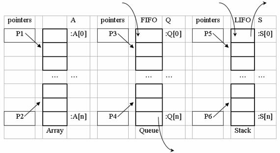
Fig. 6. Queue and stack models

On a stack, the entry point (pointed in fig. 6 by the P5) coincides with the exit point (pointed in fig. 6 by the P5). New information arrives in stack by his entry point and the stack will cumulates an element. An operation is required: the modification of P5 pointed address (in fig. 6 P5 will point to the previous element of the array). Information goes away from stack by this exit point and the stack will lose an element. An operation is required: the modification of P5 pointed address (in fig. 6 P5 will point to the subsequent element of the array). The queue it operates on LIFO (last in first out) mechanism described above.

A list can operate if the element of list will contain both the information and a pointer (see fig. 7). A list can contain more than one element. In list are linked the elements through pointer field of them (fig. 8). The last element of a list contains a zero value (called usually NULL). This is the indicator of list ending. The address of the first element of the list is stored into a pointer (P in fig. 8, called head of the list). The lists elements do not necessary occupy consequently memory addresses. As we can observe from fig. 8, the default mechanism that a list implements it is LIFO. A new element can be added to the list through three operations, depicted in fig. 9.

Fig. 7. List elements structure

Fig. 8. A list

Fig. 9. Adding of a new element to a list

A close (or circular) list does not contain a zero pointer value. Is replaced the NULL value from the end of list (see fig. 8) by the value stored in P (fig. 10). An immediate property of a close list is that it does not have a first element, because P can point on any element without losing the information.

Fig. 10. Circular lists

The procedure of element adding onto a circular list must follow the scheme depicted in figure 11.

Fig. 11. Adding a new element to a circular list

A more complex list-type structure is double-linked list. An element of a double-linked list stores the information and has two fields for pointers storing. Similar with circular lists, a double-linked list has no head. Any element of the double-linked list can act as head. An element adding procedure to a double-linked list must follow a mechanism as we describes in fig 12.

Fig. 12. Double-linked list element and inserting a new element in a double-linked list

A double linked list can be linear or circular one, but for both are enough for list management a single pointer to store an element address from the list.

Fig. 13. Binary tree element and structure

Another application of structured elements with two pointers is binary trees. A tree has one special element has act as root (of which address is stored for tree management) and every tree element has two ramifications towards another elements or NULL addresses.

A tree is not necessary complete (see fig. 13). Based on links established onto tree elements, a tree has levels. First level it contain the tree root, and the last level contain all elements situated at a distance equal with maximum distance walked by links from root element. Sow, can be counted two parameters on trees: the number of elements and the number of levels. An equilibrated tree if it contains a minimum number of levels according with his number of elements. If the tree has N levels, to be an equilibrated one, his minimum number of elements it must be 2^N-1. The terminal links of a tree (links of leafs) can be used to point somewhere in tree.

Fig. 14. Accessing superior levels from tree leafs

As example, in fig. 14 are suggested a mode to accessing previous level (parent node) from left free links and root level from right free links. More complex than binary trees are b-trees (where b value can be 3, 4 and so on). We can add a flexible mechanism of links management to the b-trees implementation (see fig. 15). A pointer to an array of pointers can serve as link point.

Fig. 15. Flexible mechanism of links management to the b-trees

A mechanism as we describes in fig. 15 allow us to create also a hybrid tree with elements with 1 link, elements with 2 links, elements with 3 links and so on.

References