Binomial Distribution Sample Confidence Intervals Estimation
3. Post and Pre Test Odds
Sorana BOLBOACĂ, Andrei ACHIMAŞ CADARIU
“Iuliu Haţieganu” University of Medicine and Pharmacy, Cluj-Napoca, Romania
Abstract
When a diagnostic test results are dichotomous a 2´2 contingency table can be create, and some indices can be compute according to the method in which the data were collected. The posttest odds is define as the odds that the patient has the target disorder, after the test is carry out. Posttest odd is a point estimator of a diagnostic test and must be accompanying by a confidence intervals in order to be correctly interpret. The paper introduces some new methods of computing confidence intervals for post and pre test odds and presents theirs performances.
In order of assessing the methods, a PHP program was creates. A set of criterions was uses in order to assess implemented methods: the average of the experimental errors, the standard deviations, and the deviation relative to the imposed significance level (α = 5%). The methods were also assessed using random values from 4 to 1000.
The experimental results shows that the Logit and Binomial methods obtained the lowest standard deviation while the Clopper-Pearson method obtained the closed average of the experimental error to the imposed significance level (α = 5%).
Keywords
Confidence intervals; Posttest odds; Pretest odds; Diagnostic test assessment
Introduction
When we looked at a diagnostic study a lot o parameters can be measured based on 2´2 contingency table depending on how the data were collected. Assessing the diagnostic studies suppose to look at the point estimation and at its confidence intervals.
The posttest odds are defines as "the odds that the patient has the target disorder after the test is carried out (pre-test odds x likelihood ratio)" [1]. In order to define posttest odds is necessary to define the next parameters:
· Pre-test odds: "the odds that the patient has the target disorder before the test is carried out (pre-test probability/[1 – pre-test probability])" [1];
· Pre-test probability: "the proportion of people with the target disorder in the population at risk at a specific time (point prevalence) or time interval (period prevalence)" [2];
· Likelihood ratio: "the likelihood that a given test results would be expected in a patient with the target disorder compared with the likelihood that the same result would be expected in a patient without the target disorder" [1], [3].
Even if for some of the diagnostic parameters are defined method for computing confidence intervals, for the post test odds we did not found any methods [4], [5], [6].
The aim of this paper was a comprehensive study of computing confidence intervals for X/(n-X) fraction (post test odds, pre test odds).
Materials and Methods
Usually, in a 2´2 contingency table there are defined four groups of patients (cases):
· real positive cases (patients with diseases and a positive test result), usually noted with a;
· false positive cases (patients which do not present the disease but have a positive test results), usually noted with b;
· false negative cases (patients which present the disease but have a negative test result), usually noted with c;
· true negative cases (patient which do not present the disease and have a negative test result), usually noted with d.
If we looked at the definition of the posttest odds for example, using following substitutions: a = X and b = n-X the mathematical formula for posttest odds (PTO) is:
![]() (1)
(1)
where X is a binomial variable.
We will find the same formula for pre test odds if the substitutions will be as follows: a + c = X, and a + b + c + d = n. The post test odds and the pre test odds can be express mathematically as X/(n-X) fraction (function named ci2 in our program [7]).
If we transform the equation (1) by dividing with X, PTO becomes:
![]() (2)
(2)
The equation (2) leads us to the mathematical expression, which uses the CI’s for proportion (X/n), in order to express the CI’s for PTO:
 (3)
(3)
where CIL is lower bound of proportion like (X/n) confidence interval, and CIU is upper bound. Using of (3) allow us to compute the confidence interval for PTO (eq. 1).
Estimating of confidence intervals for ci2 function type medical parameters like based on the literature definitions and on our experience in confidence intervals estimation, all functions defined to the proportions and proportion-like medical parameter (see paper [8]) functions were investigated.
In order to obtained a 100·(1-α) = 95% confidence intervals, we worked with a significance level equal with α = 5% (parameter noted with a in our PHP modules) and its corresponding normal distribution percentile z1-α/2 = 1.96 (noted z in our program) [7]. The sequences of the program where the above-described parameters is:
define("z",1.96); define("a",0.05);
We used as quantitative descriptors of methods performance the standard deviation of the experimental errors as well as the deviation of the experimental errors relative to the imposed significance level (α = 5%). The standard deviation of the experimental error (StdDev) was computes using the next formula:
 (4)
(4)
where StdDev(X) is standard deviation, Xi is the experimental errors for a given i, M(X) is the arithmetic mean of the experimental errors and n is the sample size.
If we have a sample of n elements with a known (or expected) mean (equal with 100α), the deviation around α = 5% (imposed significance level) is giving by:
 (5)
(5)
The best value of Dev5 for a given n gives us the best method of computing the confidence intervals for specified sample size (n) if we looked after a method with the smallest deviation.
The performance of each method for different sample sizes (n) and different values of binomial variable (X) was asses using a set of criterions. First, were computes and graphically represented the ci2 function, the lower and upper confidence boundaries using six methods, at a sample size equal with 10 (n = 10):
$c_i=array( "Wilson" , "Logit" , "LogitC" , "BayesF" , "Jeffreys" , "Binomial" );
define("N_min",10);define("N_max",11); est_ci_er(z,a,$c_i,"R","ci2","ci");
· using sixteen methods when the sample size (n) was varying from 4 to 103. The values of the post test odds and the lower and upper confidence intervals boundaries were computed with the next sequence of the program:
$c_i=array( "Wald", "WaldC", "Wilson", "WilsonC", "ArcS", "ArcSC1", "ArcSC2",
"ArcSC3", "AC", "Logit", "LogitC", "BS", "Bayes", "BayesF", "Jeffreys", "CP" );
define("N_min",4); define("N_max",104); est_ci_er(z,a,$c_i,"R","ci2","ci");
The graphical representation for samples size varying from 4 to 103 for ci2 function (X/(n-X)), and for the upper and lower confidence boundaries were obtained using a graphical module implemented in PHP [7].
Second, the average and standard deviation (StdDev) of the experimental errors, the deviation relative to imposed significance level (Dev5) for a list of sample sizes (n =10, 50, 100, 300, and 1000):
$c_i=array("LogitC", "BayesF", "Wilson" , "Logit" , "Jeffreys" , "Binomial" );
· For n = 10: define("N_min",10); define("N_max",11); est_ci_er(z,a,$c_i,"R","ci2","er");
· for n = 50 was modified as follows: define("N_min",50); define("N_max",51);
· For n = 100 was modified as follows: define("N_min",100);define("N_max",101);
· For n = 300 was modified as follows: define("N_min",300);define("N_max",301);
· For n = 1000 was modified as follows: define("N_min",1000);define("N_max",1001);
The results, was imported in Microsoft Excel, where were created the graphical representations of the dependency of percentage of the experimental errors and X variable depending on n. In the graphical representation, on horizontal axis were represented the n values depending on X binomial distribution variable and on the vertical axis the percentage of the experimental errors.
Third, the average of experimental errors and standard deviations (StdDev) when the sample size varies from 4 to 100 were compute using the next sequence of the program:
$c_i=array("LogitC", "BayesF", "Wilson" , "Logit" , "Jeffreys" , "Binomial" );
define("N_min",4); define("N_max",101); est_ci_er(z,a,$c_i,"R","ci2","er");
Fourth, we computed the experimental errors and the deviation relative to the imposed significance level (Dev5)) for each method when the sample size varies from 4 to 103. The sequence of the program used was:
$c_i=array("Wald","WaldC","Wilson","WilsonC","ArcS","ArcSC1","ArcSC2","ArcSC3",
"AC","CP", "Logit", "LogitC", "Bayes", "BayesF", "Jeffreys","Binomial");
define("N_min",4);define("N_max",103);
· For experiemental errors:
est_ci_er(z,a,$c_i,"R","ci2","er");
· For variation relative to the imposed significance level was modifierd:
est_ci_er(z,a,$c_i,"R","ci2","va");
Fifth, the performance of sixteen methods were assesed on a 100 random numbers for binomial variable (X) and sampel size (n), when 0 < X < n and 4 ≤ n ≤ 1000. The sequence of the program is:
$c_i=array("Wald","WaldC","Wilson","WilsonC","ArcS","ArcSC1","ArcSC2","ArcSC3",
"AC","CP", "Bayes", "BayesF", "Jeffreys", "Logit", "LogitC", "Binomial");
define("N_min", 4); define("N_max",1000); est_ci_er(z,a,$c_i,"ci2","ra");
Results
The contour plots of the ci2 function and its lower and upper confidence boundaries using a confidence intervals method based on binomial distribution are in figure 1, and were creates using an original PHP graphic module. With red color was represented the values 0, with yellow the values 0.5 and with blue the values 1. The intermediary color between the couplets colors were represented used 18 hue (9 hues for each combination between three colors from the couplet).
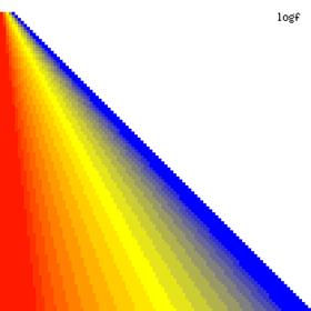
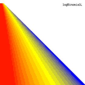
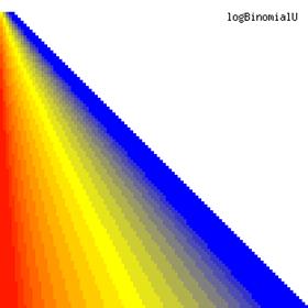
Figure 1. The contour plot for the posttest odds values and its confidence boundaries computed based on original Binomial method
The confidence boundaries of ci2 function-type at n = 10 were obtained and graphically represented (figure 2). The experimental results serve for graphical representations, which were creates.
The lower boundaries (in logarithmical scale) for a given X and a sample size equal with 10 (n = 10), for each choused method (Wilson, Logit, LogitC, BayesF, Jeffreys, and Binomial) were graphical represented in the figure 2.
Figure 2. The lower boundaries of confidence intervals for post test odds where 1 ≤ X ≤ n/2
at n = 10 (logarithmical scale depending on X)
The percentage of experimental errors for specified sample size and specified methods, are in figure 3 (for sample size equal with 10), figure 4 (for sample size equal with 50), figure 5 (for sample size equal with 100), figure 6 (for sample size equal with 300), and figure 7 (for sample size equal with 1000).
The average of experimental errors (MErr) and experimental standard deviations (StdDev) according to the sample size (n) are in table 1.
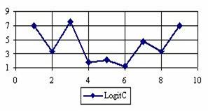

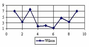
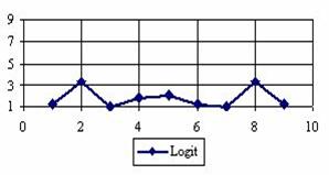
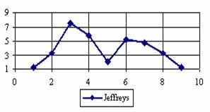

Figure 3. The percentages of the experimental error for ci2 function at n = 10 (0 < X < n)
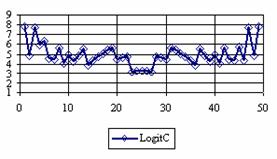
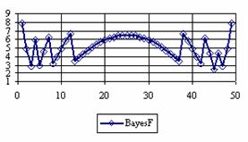
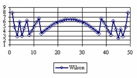
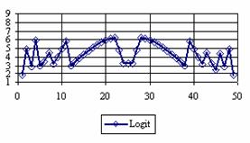
Figure 4. The percentage of the experimental error for ci2 at n = 50 (0 < X < n)
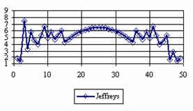
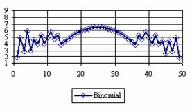
Figure 4. The percentage of the experimental error for ci2 at n = 50 (0 < X < n)
Figure 5. The percentages of the experimental error for ci2 function at n=100 (0 < X < n)

Figure 6. The percentages of the experimental error for ci2 function at n = 300 (0 < X < n)
Figure 6. The percentages of the experimental error for ci2 function at n = 300 (0 < X < n)
Figure 7. The percentage of the experimental error for ci2 function at n = 1000 (0 < X < n)
n |
Method |
LogitC |
BayesF |
Wilson |
Binomial |
Logit |
Jeffreys |
|
10 |
MErr |
4.22 |
4.22 |
4.22 |
3.84 |
1.81 |
3.84 |
|
StdDev |
2.45 |
2.45 |
2.45 |
2.17 |
0.90 |
2.17 |
|
|
50 |
MErr |
4.94 |
5.13 |
5.13 |
4.88 |
4.35 |
5.03 |
|
StdDev |
1.13 |
1.31 |
1.31 |
1.12 |
1.23 |
1.47 |
|
|
100 |
MErr |
5.20 |
5.05 |
5.05 |
4.96 |
4.69 |
4.96 |
|
StdDev |
0.81 |
0.91 |
0.98 |
0.80 |
0.93 |
1.03 |
|
|
300 |
MErr |
5.03 |
4.99 |
4.98 |
5.00 |
4.85 |
5.02 |
|
StdDev |
0.73 |
0.75 |
0.76 |
0.65 |
0.74 |
0.79 |
|
|
1000 |
MErr |
5.01 |
5.00 |
4.98 |
5.00 |
4.92 |
5.01 |
|
StdDev |
0.44 |
0.43 |
0.45 |
0.37 |
0.45 |
0.46 |
Table 1. The average of the experimental errors and standard deviations
at n = 10, 50, 100, 300 and 1000
The averages (MErr) and standard deviations (StdDev) of the experimental errors when n vary from 4 to 103 are in table 2.
|
Method |
Wilson |
Logit |
LogitC |
BayesF |
Jeffreys |
Binomial |
|
MErr (StdDev) |
4.7 (1.5) |
4.2 (1.3) |
4.8 (1.4) |
4.7 (1.5) |
4.6 (1.5) |
4.5 (1.3) |
Table 2. Averages and standard deviations of the experimental errors for ci2 function at 4 ≤ n < 104
The contour plots of experimental errors when sample size (n) varies from 4 to 103 were illustrated in figure 8. On the plots were represented the experimental errors from 0% (red color) to 5% (yellow color) and ≥10% (blue color) using 18 intermediate hues. The vertical axis represents the n values and the horizontal axis the X values (from 0 to n).
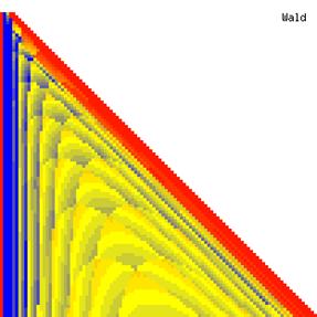
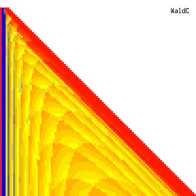
Figure 8. The contour plot of the experimental errors for ci2 function at 3 < n < 104
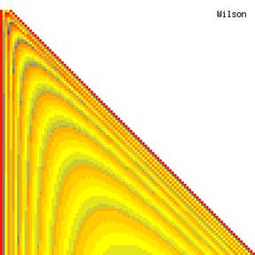
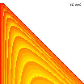
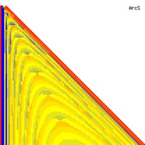
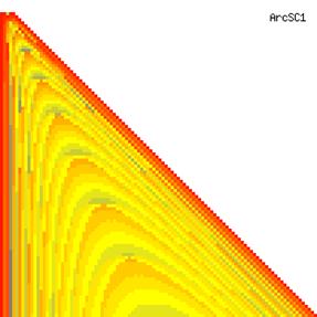
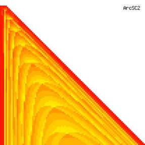
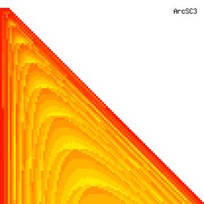
Figure 8. The contour plot of the experimental errors for ci2 function at 3 < n < 104
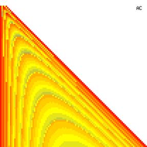
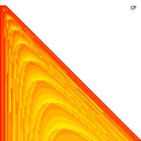
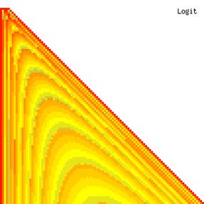
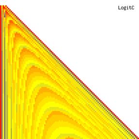
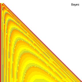
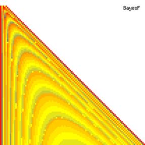
Figure 8. The contour plot of the experimental errors for ci2 function at 3 < n < 104
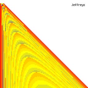
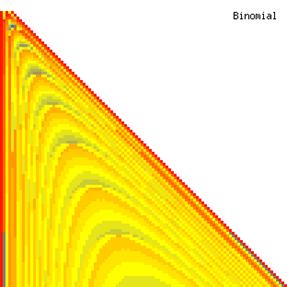
Figure 8. The contour plot of the experimental errors for ci2 function at 3 < n < 104
Using the function (3) presented in materials and methods as classification criteria, the graphical representation of frequencies of the best deviation relative to the imposed significance level (α = 5%) was obtained and depicted in figure 9.
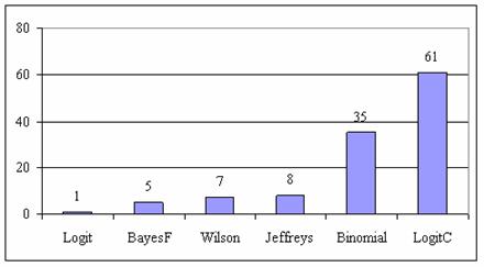
Figure 9. The best deviation frequencies of the experimental error relative to significance level (α = 5%) for posttest odds at n = 4...103
The results of the deviations relative to the imposed significance level (α = 5%) when the sample size vary (104 ≤ n ≤ 109) are in table 3.
n |
Binomial |
LogitC |
Jeffreys |
BayesF |
|
104, 105 |
0.89, 0.82 |
0.88, 0.88 |
1.09, 1.04 |
1.03, 1.02 |
|
106, 107 |
0.83, 0.82 |
0.88, 0.87 |
1.04, 1.03 |
1.02, 1.01 |
|
108, 109 |
0.81, 0.81 |
0.86, 0.88 |
1.02, 1.01 |
1.01, 1.00 |
Table 3. The deviations relative to the significance level for ci2 function at 104 ≤ n ≤109
· Based on the results from the random values of binomial variable (X; 1≤ X <n) and sample size (n; 4 ≤ n ≤ 1000), a set of calculation were performed and graphical represented in figure 10.
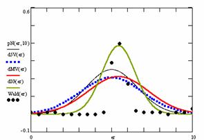
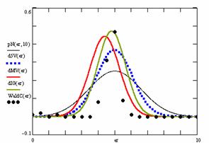
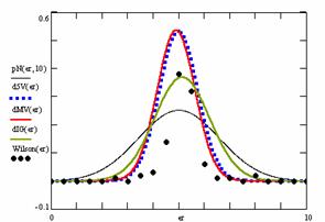
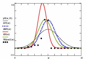
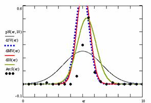
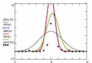
Figure 10. The pN(er, 10), d5V(er), dMV(er), dIG(er) and the frequencies of the experimental errors for each specified method for random X, n (1 ≤ X < 1000, 4 ≤ n ≤ 1000)
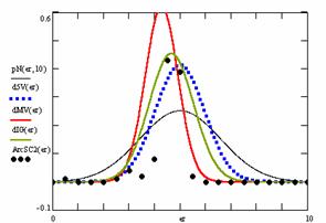
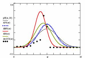
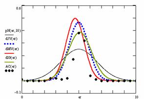
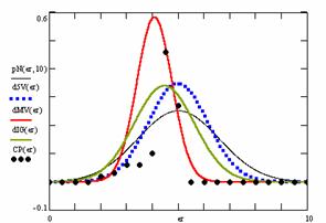
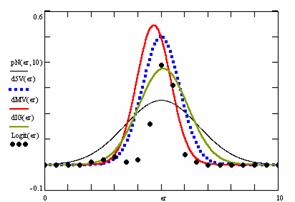
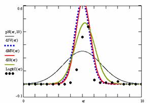
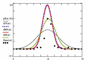
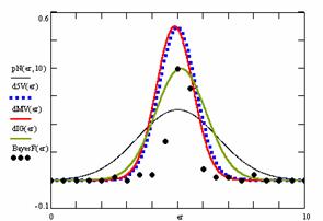
Figure 10. The pN(er, 10), d5V(er), dMV(er), dIG(er) and the frequencies of the experimental errors for each specified method for random X, n (1 ≤ X < 1000, 4 ≤ n ≤ 1000)
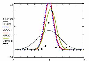
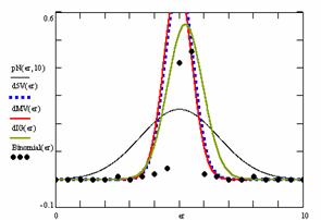
Figure 10. The pN(er, 10), d5V(er), dMV(er), dIG(er) and the frequencies of the experimental errors for each specified method for random X, n (1 ≤ X < 1000, 4 ≤ n ≤ 1000)
In the figure 10 are:
· The frequencies of the experimental error (black dots) for each specified method;
· dIG(er): the best errors interpolation curve with a Gauss curve (green line);
· dMV(er): the Gauss curves of the average and standard deviation of the experimental errors (red line);
· d5V(er): the Gauss curve of the experimental errors deviations relative to the significance level (blue squares);
· pN(er,10): the Gauss curve of the standard binomial distribution (black line) from the average of the errors equal with 5.
For the random samples, the results are in tables 4 to 7.
Table 4 contains the average of the deviation of the experimental errors relative to significance level α =5% (Dev5), the absolute differences of the average of experimental errors relative to the imposed significance level (|5-M|), and standard deviations (StdDev).
Table 5 contains the absolute differences of the averages that result from Gaussian interpolation curve to the imposed significance level (|5-MInt|), the deviations that result from Gaussian interpolation curve (DevInt), the correlation coefficient of interpolation (r2Int) and the Fisher point estimator (FInt).
The superposition of the standard binomial distribution curve and interpolation curve (pNIG), the superposition of standard binomial distribution curve and the experimental error distribution curve (pNMV), and the superposition of standard binomial distribution curve and the error distribution curve around significance level (α = 5%) (pN5V) were presented in table 6.
|
No |
Method |
Dev5 |
Method |
|5-M| |
Method |
StdDev |
|
1 |
ArcS |
0.55 |
CP |
0.02 |
LogitC |
0.60 |
|
2 |
ArcSC1 |
0.55 |
WilsonC |
0.05 |
Binomial |
0.61 |
|
3 |
Binomial |
0.56 |
Bayes |
0.07 |
ArcSC1 |
0.62 |
|
4 |
LogitC |
0.63 |
Logit |
0.08 |
Jeffreys |
0.65 |
|
5 |
Jeffreys |
0.64 |
ArcSC3 |
0.08 |
CP |
0.72 |
|
6 |
Bayes |
0.69 |
Wald |
0.08 |
AC |
0.73 |
|
7 |
BayesF |
0.73 |
Wilson |
0.10 |
Logit |
0.74 |
|
8 |
Wilson |
0.75 |
WaldC |
0.11 |
ArcSC2 |
0.74 |
|
9 |
Logit |
0.80 |
AC |
0.30 |
Bayes |
0.76 |
|
10 |
AC |
0.86 |
ArcS |
0.31 |
BayesF |
0.76 |
|
11 |
ArcSC2 |
0.96 |
Jeffreys |
0.43 |
Wilson |
0.76 |
|
12 |
WilsonC |
1.06 |
BayesF |
0.60 |
ArcSC3 |
0.76 |
|
13 |
WaldC |
1.08 |
ArcSC2 |
0.72 |
WilsonC |
0.83 |
|
14 |
CP |
1.15 |
Binomial |
0.82 |
WaldC |
1.08 |
|
15 |
ArcSC3 |
1.27 |
ArcSC1 |
0.92 |
ArcS |
1.23 |
|
16 |
Wald |
1.93 |
LogitC |
0.96 |
Wald |
1.69 |
Table 4. Methods ordered by performance according to Dev5, |5-M| and StdDev criterions
|
No |
Method |
|5-MInt| |
Method |
DevInt |
Method |
r2Int |
FInt |
|
1 |
Logit |
0.09 |
Binomial |
0.72 |
ArcSC3 |
0.64 |
35 |
|
2 |
AC |
0.10 |
ArcS |
0.79 |
CP |
0.64 |
35 |
|
3 |
BayesF |
0.13 |
Jeffreys |
0.79 |
WilsonC |
0.69 |
43 |
|
4 |
Wilson |
0.14 |
ArcSC1 |
0.83 |
Wald |
0.69 |
43 |
|
5 |
Bayes |
0.14 |
WaldC |
0.84 |
Logit |
0.71 |
47 |
|
6 |
WaldC |
0.18 |
ArcSC2 |
0.85 |
Wilson |
0.72 |
48 |
|
7 |
LogitC |
0.22 |
LogitC |
0.85 |
BayesF |
0.72 |
49 |
|
8 |
Binomial |
0.25 |
BayesF |
0.99 |
AC |
0.72 |
50 |
|
9 |
ArcSC1 |
0.28 |
Bayes |
1.00 |
Bayes |
0.72 |
50 |
|
10 |
Jeffreys |
0.30 |
AC |
1.03 |
ArcSC2 |
0.73 |
51 |
|
11 |
ArcSC2 |
0.33 |
Wald |
1.03 |
Jeffreys |
0.73 |
51 |
|
12 |
ArcS |
0.35 |
WilsonC |
1.04 |
LogitC |
0.74 |
54 |
|
13 |
WilsonC |
0.43 |
Logit |
1.06 |
WaldC |
0.74 |
55 |
|
14 |
Wald |
0.45 |
Wilson |
1.08 |
ArcSC1 |
0.75 |
56 |
|
15 |
ArcSC3 |
0.54 |
CP |
1.17 |
ArcS |
0.75 |
57 |
|
16 |
CP |
0.54 |
ArcSC3 |
1.21 |
Binomial |
0.75 |
58 |
Table 5. Methods ordered by |5-Mint|, DevInt, r2Int and FInt criterions
|
No |
Method |
pNIG |
Method |
pNMV |
Method |
pN5V |
|
1 |
Binomial |
0.63 |
ArcS |
0.52 |
ArcS |
0.53 |
|
2 |
Jeffreys |
0.65 |
ArcSC1 |
0.53 |
ArcSC1 |
0.53 |
|
3 |
ArcS |
0.66 |
Binomial |
0.54 |
Binomial |
0.54 |
|
4 |
ArcSC1 |
0.69 |
CP |
0.54 |
LogitC |
0.58 |
|
5 |
WaldC |
0.70 |
WilsonC |
0.54 |
Jeffreys |
0.59 |
|
6 |
LogitC |
0.70 |
ArcSC2 |
0.54 |
Bayes |
0.62 |
|
7 |
ArcSC2 |
0.71 |
LogitC |
0.58 |
BayesF |
0.65 |
|
8 |
Wald |
0.77 |
Jeffreys |
0.58 |
Wilson |
0.65 |
|
9 |
WilsonC |
0.77 |
ArcSC3 |
0.59 |
Logit |
0.68 |
|
10 |
BayesF |
0.78 |
Bayes |
0.62 |
AC |
0.71 |
|
11 |
Bayes |
0.78 |
Logit |
0.63 |
ArcSC2 |
0.77 |
|
12 |
AC |
0.80 |
BayesF |
0.64 |
WilsonC |
0.81 |
|
13 |
CP |
0.80 |
Wilson |
0.65 |
WaldC |
0.82 |
|
14 |
Logit |
0.81 |
AC |
0.67 |
CP |
0.85 |
|
15 |
ArcSC3 |
0.81 |
WaldC |
0.69 |
ArcSC3 |
0.89 |
|
16 |
Wilson |
0.81 |
Wald |
0.88 |
Wald |
0.90 |
Table 6. The confidence intervals methods ordered by the
pIGMV, pIG5V, and pMV5V criterions
|
No |
Method |
pIGMV |
Method |
pIG5V |
Method |
pMV5V |
|
1 |
Jeffreys |
0.86 |
AC |
0.90 |
ArcSC1 |
0.99 |
|
2 |
LogitC |
0.83 |
WaldC |
0.86 |
Binomial |
0.96 |
|
3 |
BayesF |
0.82 |
Logit |
0.86 |
Bayes |
0.96 |
|
4 |
WaldC |
0.81 |
ArcSC2 |
0.85 |
LogitC |
0.95 |
|
5 |
Bayes |
0.80 |
BayesF |
0.84 |
Jeffreys |
0.95 |
|
6 |
Wilson |
0.80 |
WilsonC |
0.84 |
Wilson |
0.95 |
|
7 |
AC |
0.80 |
ArcSC3 |
0.83 |
ArcS |
0.94 |
|
8 |
Binomial |
0.79 |
Jeffreys |
0.82 |
BayesF |
0.94 |
|
9 |
ArcS |
0.77 |
CP |
0.82 |
Wald |
0.90 |
|
10 |
ArcSC1 |
0.77 |
LogitC |
0.82 |
AC |
0.85 |
|
11 |
ArcSC2 |
0.76 |
Wilson |
0.82 |
Logit |
0.83 |
|
12 |
ArcSC3 |
0.76 |
Binomial |
0.82 |
WaldC |
0.75 |
|
13 |
Logit |
0.76 |
Bayes |
0.81 |
ArcSC2 |
0.63 |
|
14 |
WilsonC |
0.73 |
ArcSC1 |
0.76 |
ArcSC3 |
0.61 |
|
15 |
Wald |
0.72 |
ArcS |
0.74 |
WilsonC |
0.60 |
|
16 |
CP |
0.71 |
Wald |
0.69 |
CP |
0.57 |
Table 7. The confidence intervals methods ordered by the
pIGMV, pIG5V, and pMV5V criterions
Table 7 contains the superposition of interpolation Gauss curve and the Gauss curve of error around experimental mean (pIGMV); the interpolation Gauss curve and the Gauss curve of error around imposed mean (pIG5V); and the Gauss curve of experimental error around experimental mean and the error Gauss curve around imposed mean α = 5% (pMV5V).
Discussions
Looking at the sample size equal with 50 we can observed (figure 4) that the percentage of the experimental errors obtained by the Logit method were systematically under the imposed significance level (α = 5%) with an average of the experimental errors equal with 1.8%. The average of the experimental errors for Jeffreys and Binomial methods were equal with 3.8%. The less value for standard deviation was obtains by the Binomial method. We can observe from the table 1 that the Binomial method obtained the lowest standard for 100 ≤ n ≤ 1000.
If we looked at the behaviors of the methods used in computing the confidence interval for ci2 function at a sample size equal with 300 we can observed (figure 5) that the experimental errors obtained with Logit and Jeffreys, for X closed to 0 and closed to 100 were significantly lower comparing with the imposed significance level (α = 5%). To the extremities of the X (0, n), the other methods (Wilson, Logit, BayesF, Binomial) obtained experimental errors greater than the imposed significance level (α = 5%).
Looking at the experimental errors from a sample size equal with 300 and 1000 (figure 6 and 7) we cannot said that there were any differences between confidence intervals estimation errors. Thus, we can say that the osculation of the experimental errors obtained with Binomial and the Jeffreys methods were not so ample compared with the other confidence intervals estimations.
Analyzing the figure 9 some aspects were disclosure. The first observation was that the method LogitC obtained the best performance followed by the original method Binomial. The original method, named Binomial, improved the BayesF and the Jeffreys methods even if to the limit the Binomial method overlap on BayesF and Jeffreys methods (see the Binomial function):
![]() ,
, ![]()
The second observation was that amongst binomial methods, the original Binomial method obtained best performances (with 35 apparitions, followed by Jeffreys with 8 apparitions).
The third observation which can be observed just from the experimental data (cannot been seen from the graphical representation) was that for n > 85 the Binomial method was almost systematically the method with the lowest standard deviation. In order to confirm that for n ≥ 85 the Binomial method obtains the best deviation relative to the imposed significance level, six sample sizes from 104 to 109 uses to compute the errors. The experimental data from the table 3 confirm the hypothesis that Binomial method obtain the lowest deviation relative to the significance level α = 5%. As it can be observes, the errors deviation of the Binomial method was lower compared with the other methods (see table 3).
The best three confidence intervals methods reported to the sample size (n) at a significance level equal with 5% were:
· for n = 10: LogitC, BayesF, Wilson;
· for n = 50: LogitC, Binomial, BayesF, Wilson;
· for n = 100: Binomial, BayesF, Wilson;
· for n = 300: Binomial, LogitC, BayesF;
· for n = 1000: Binomial, BayesF, LogitC.
If we looked at the results obtained from the random samples (X, n random numbers from 4 to 1000) we can remarked that the Clopper-Pearson method obtained the closed experimental error average to the significance level (α = 5%) (table 4); the lowest experimental standard deviation were obtained by the LogitC and Binomial methods. The most closed experimental standard deviation to the imposed significance level (α = 5%) was obtained by the ArcS method followed by the ArcSC1, Binomial and LogitC methods.
The Logit method obtained the closed interpolation average to the significance level (table 5), followed by the Agresti-Coull method; Binomial was the method with the lowest interpolation standard deviation. The best correlation between theoretical curve and experimental data are obtains by the Binomial method followed by the ArcS method.
The Wilson method, obtained the maximum superposition between the curve of interpolation and the curve of standard binomial distribution (figure 6). The maximum superposition between the curve of standard binomial distribution and the curve of experimental errors was obtained by the Wald method, method which obtained also the maximum superposition between the curve of standard binomial distribution and the curve of errors around the significance level (α = 5%).
The maximum superposition between the Gauss curve of interpolation and the Gauss curve of errors around experimental mean was obtains by the Jeffreys method, followed by the LogitC, and the BayesF methods (table 7). The Agresti-Coull method obtained the maximum superposition between the Gauss curve of interpolation and the Gauss curve of errors around significance level, followed by the LogitC method. The maximum superposition between the Gauss curve of experimental error and the Gauss curve of errors around imposed mean were obtains by the ArcSC1 method closely followed by the Binomial and the Bayes methods.
Conclusions
Choosing of the confidence intervals methods for ci2 function is a difficult task. The Logit (for n = 10) and the LogitC methods (for n = 50) were more conservative compared with the other methods if we were looked at the standard deviation of the experimental errors (at a significance level of α = 5%). Systematic, for 100 ≤ n ≤ 1000 the Binomial method obtained the most conservative standard deviation of the experimental errors and always the average of the experimental errors less than choused significance level (α = 5% for our experiments).
The LogitC and Binomial methods obtains the lowest standard deviation of the experimental errors on random samples (0 < X < n and 4 ≤ n ≤ 1000) and the Clopper-Pearson method obtained the closed average of the experimental error to the imposed significance level (α = 5%).
Acknowledgements
The first author is thankful for useful suggestions and all software implementation to Ph. D. Sci., M. Sc. Eng. Lorentz JÄNTSCHI from Technical University of Cluj-Napoca.
References