Binomial Distribution Sample Confidence Intervals Estimation

4. Post Test Probability

 

Sorana BOLBOACĂ, Andrei ACHIMAŞ CADARIU

 

“Iuliu Haţieganu” University of Medicine and Pharmacy, Cluj-Napoca, Romania

sbolboaca@umfcluj.ro

 

 

Abstract

Posttest probability is one of the key parameters which can be measured and interpret in dichotomous diagnostic tests. Defined as the proportion of patients, which present particular test result and the target disorder, the posttest probability is a parameter used in assessing the efficiency of the diagnostic. As a point estimated parameter, posttest probability needs a confidence interval in order to interpreting trustworthiness or robustness of the finding. Unfortunately, for post test probability there was no confidence intervals reported in literature. The aim of this paper is to introduce six methods named Wilson, Logit, LogitC, BayesF, Jeffreys, and Binomial as methods of computing confidence intervals for posttest probability and to present theirs performances.

Computer implementations of the methods use the PHP language. The performance of each method for different sample sizes and different values of binomial variable was asses using a set of criterions. One criterion was the average of experimental errors and standard deviations. Second, the deviation relative to imposed significance level (α = 5%). Third, the behavior of the methods when the sample size vary from 4 to 103 and on random sample and random binomial variable in 4..1000 domain.

The results of the experiments show us that the Binomial method obtain the best performances in computing the confidence intervals for posttest probability for sample size starting with 36.

 

 

Keywords

Confidence intervals estimation; binomial distribution; Posttest probability; Diagnostic test assessment

 

 

Introduction

 

The simplest diagnostic studies generate dichotomous results when the patients can be classifying according to the presence or absence of disease. In this case, a lot of key parameters of interest can be compute in order to measure the effect size of the diagnostic test: sensitivity, specificity, predictive positive value, negative predictive value, pre test probability, post test probability, pre test odds and so on [1], [2], [3], [4]. Whatever the parameters are, some assessment must be made of the trustworthiness or robustness of the finding [5].

The finding of a medical study can provide a point estimation of effect and nowadays is necessary that the point estimation to have a confidence intervals which to allow us to interpret correctly the point estimation of an interest parameter. Unfortunately, for post test probability there was no confidence intervals reported in literature [2], [6], [7], [8], [9], [10].

The post test probability was defined as: ״the proportion of patients with that particular test result who have the target disorder (posttest odds/[1 + post-test odds])״ [3].

The aim of this paper is to introduce six methods named Wilson, Logit, LogitC, BayesF, Jeffreys, and Binomial as methods of computing confidence intervals for posttest probability and to present theirs performances.

 

           

Materials and Methods

 

            In a 2 by 2 contingency tables, according with the presence or absence of a disease and a positive or negative test results, the patients can be classifies in four groups. First group, patients with diseases and a positive test result (real positive cases), noted usually with a. Second group, patients which do not present the disease but have a positive test results (false positive cases) usually noted with b. Third group, patients which present the disease but have a negative test result (false negative cases) usually noted with c. The fourth group, patient that do not present the disease and have a negative test result (true negative cases) usually noted with d.

Using following substitutions: a = X, b = n-X, c = Y, d = m-Y, (X and Y are independent binomial distribution variables of sizes m and n), the posttest probability (PTP) becomes:

                                                                               (1)

Thus, we can say that from mathematical point of view the post test probability parameter is of X/(2X-n) function type, function named ci3 in our program [11].

The function ci3(X, n) = f(X) = X/(2X-n) present an asymptotic point of variation at ±∞ at even n and X = n/2. The graphical representation of this function at n = 20 was represented in figure 1, where X was considered a continuous variable.

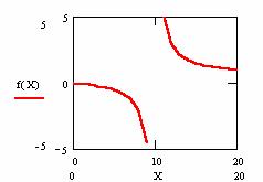
Figure 1. The dependency for continuous variation of X of the posttest probability at n = 20

 

Some of the methods, which obtained performance in confidence intervals estimation of a binomial proportion, were included in this study. The methods included in the experiment were Wilson, Logit, LogitC, BayesF, Jeffreys, and Binomial. The mathematical formulas and corresponding functions were presents in a previous paper [12].

In order to obtain a 100·(1-α) = 95% confidence intervals (is most frequently used confidence intervals) the experiments were runs at a significance level α = 5% (noted with a in our program). Corresponding to choused significance level was used its normal distribution percentile z_1-α/2 = 1.96 (noted with z in our program). The sequence of the program is: define("z",1.96); define("a",0.05);

The performance of each method for different sample sizes and different values of binomial variables was asses using a set of criterions. First, was computes upper and lower boundaries for following cases:

·        a given X (15 ≤ X ≤ 19) and a specified sample size (n = 20) for choused methods:

$c_i=array( "Wilson" , "Logit" , "LogitC" , "BayesF" , "Jeffreys" , "Binomial" );

define("N_min",20);define("N_max",21); est_ci_er(z,a,$c_i,"RD","ci3","ci");

·        a sample size varying from 4 to 103:

$c_i=array( "Wald", "WaldC", "Wilson", "WilsonC", "ArcS", "ArcSC1", "ArcSC2",

        "ArcSC3", "AC", "Logit", "LogitC", "BS", "Bayes", "BayesF", "Jeffreys", "CP" );

define("N_min",4); define("N_max",104); est_ci_er(z,a,$c_i,"RD","ci3","ci");

The contour plots represented for samples size varying from 4 to 103 for ci3 function and for the upper and lower confidence boundaries were obtained using a graphical module implemented in PHP [11].

Second, the average of experimental errors, the standard deviations of experimental errors, and  the deviation relative to imposed significance level (α = 5%). The standard deviation of the experimental error (StdDev) was computes using the next formula:

                                                                   (2)

where StdDev(X) is standard deviation, X_i is the experimental errors for a given i, M(X) is the arithmetic mean of the experimental errors and n is the sample size.

If we have a sample of n elements with a known (or expected) mean (equal with 100α), the deviation around α = 5% (imposed significance level) is giving by:

                                                                        (3)

The standard deviation of the experimental errors as well as the deviation around the imposed significance level was uses as quantitative descriptors of the methods performances.

The value of sample size (n) was chosen in the conformity with the real number from the medical studies; in our experiments, we used 10 ≤ n ≤ 300 domains (n = 20, 50, 100, 300, and 1000). The estimation of the methods was performed for the binomial value of X variable, which respect the rule: 0 < X < n. The sequence of the program that allowed us to compute the experimental errors for specified sample sizes and specified method were:

$c_i=array("LogitC", "BayesF", "Wilson" , "Logit" , "Jeffreys" , "Binomial" );

·      For n = 20: define("N_min",20); define("N_max",21); est_ci_er(z,a,$c_i,"RD","ci","er");

·      For n = 50 was modified as follows: define("N_min",50); define("N_max",51);

·      For n = 100 was modified as follows: define("N_min",100); define("N_max",101);

·      For n = 300 was modified as follows: define("N_min",300);define("N_max",301);

·      For n = 1000 was modified as follows: define("N_min",1000);define("N_max",1001);

The results were graphically represents as a dependency between error estimation and X variable depending on n. In the graphical representation, on horizontal axis were represented the n values depending on X and on the vertical axis the percentage of the experimental errors.

Third, the average of the experimental errors and standard deviations for a sample size, which vary from 4 to 103 (4 ≤ n < 104, and 0 ≤ X ≤ n) was computed using the sequence of the program:

$c_i=array("Wald","WaldC","Wilson","WilsonC","ArcS","ArcSC1","ArcSC2","ArcSC3",

       "AC", "CP", "Logit", "LogitC", "Bayes", "BayesF", "Jeffreys", "Binomial");

define("N_min",4); define ("N_max",103); est_ci_er(z,a,$c_i,"RD","ci3","er");

The contour plots of experimental errors were creates. On the contour plots were represented the error from 0% (red color) to 5% (yellow color) and ≥10% (blue color) using 18 hue. The vertical axis represents the n values (from 4 to 103) and the horizontal axis the X values (from 0 to n).

Fourth, the deviations relative to the imposed significance level (α = 5%) when the sample size vary from 4 to 103 (4 ≤ n < 104, and 0 ≤ X ≤ n) was computed. The sequence of the program is:

$c_i=array("LogitC", "BayesF", "Wilson" , "Logit" , "Jeffreys" , "Binomial" );

define("N_min",4); define ("N_max",103); est_ci_er(z,a,$c_i,"RD","ci3","va");

Fifth, the performance of sixteen methods were assesed on a 100 random numbers for binomial variable (X) and sampel size (n), when 4 ≤ X < n and 4 ≤ n ≤ 1000. The sequence of the program is:

$c_i=array("Wald","WaldC","Wilson","WilsonC","ArcS","ArcSC1","ArcSC2","ArcSC3",

       "AC", "CP", "Logit", "LogitC", "Bayes", "BayesF", "Jeffreys", "Binomial");

define("N_min", 4); define("N_max",1000); est_ci_er(z,a,$c_i,"ci3","ra");

 

 

Results

 

The confidence boundaries for ci3 function-type at n = 20 were obtained and graphically represented. The experimental results were imports in Microsoft Excel (figure 1) and in a PHP graphic module (figure 2) where the graphical representations were creates.

The lower and upper confidence intervals boundaries for a given X (15 ≤ X ≤ 19) at a sample size equal with 20 (n = 20), for each choused methods were graphical represented in the figure 1.

 

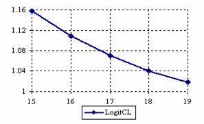
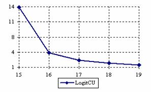
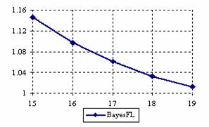
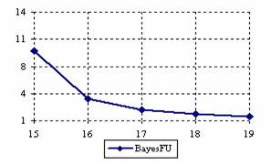
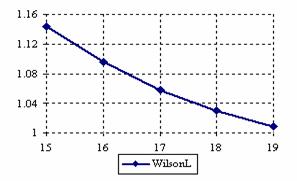
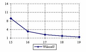
Figure 1. The lower and upper confidence boundaries for posttest probability;

(15 ≤ X ≤ 19)) at n = 20

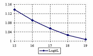
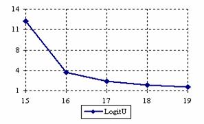
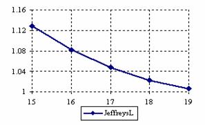
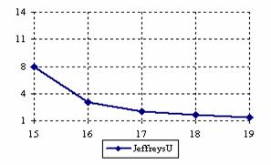
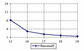
Figure 1. The lower and upper confidence boundaries for posttest probability;

(15 ≤ X ≤ 19)) at n = 20

 

The posttest probability and its lower and upper confidence boundaries were represents in the figure 2. With red color were represented the experimental values of -10, with yellow the experimental values of 0 and with blue the experimental values of 10. The color between the couplets colors were represented used 252 hue. The infinite values and the value for that the function was undefined were represented with white.

The percentages of experimental errors depending on X value (0 < X < n) for specified sample size and specified method were presented. For a sample size equal with 20, the graphical representations of the experimental errors are in figure 3.

 

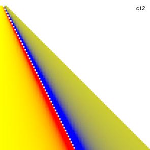
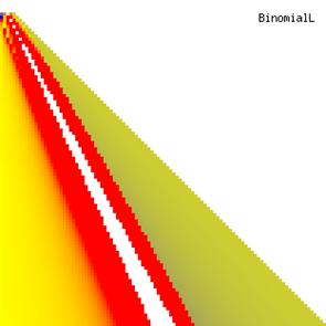
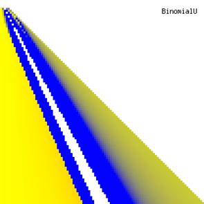
Figure 2. Level surfaces for posttest probability values and its confidence intervals boundaries computed with Binomial method

 

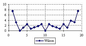
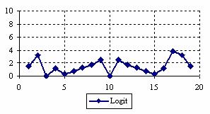
Figure 3. The percentages of the experimental errors

for posttest probability at n = 20 (0<X<n)

 

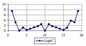
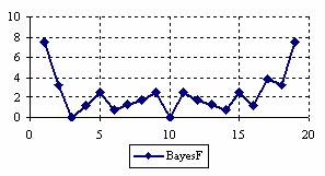
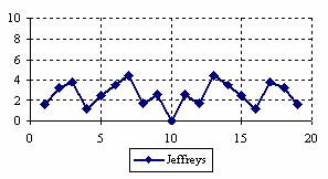
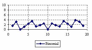
Figure 3. The percentages of the experimental errors

for posttest probability at n = 20 (0<X<n)

 

The percentages of the experimental errors for a sample size of 50 using specified method are in figure 4.

 

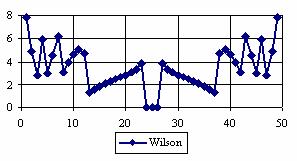
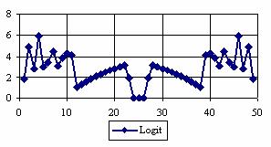
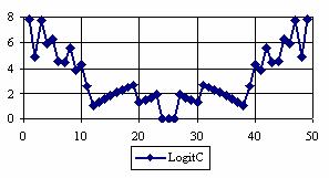
Figure 4. The percentages of the experimental errors

for posttest probability at n = 50 (0 < X < n)

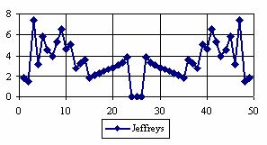
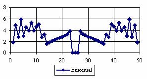
Figure 4. The percentages of the experimental errors

for posttest probability at n = 50 (0 < X < n)

 

The graphical representations of the percentage of the experimental errors for a sample size equal with 100 using specified method are in figure 5.

 

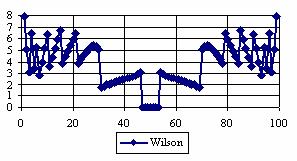
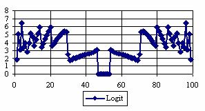
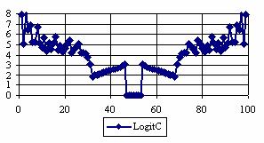
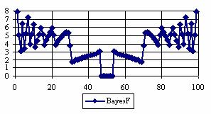
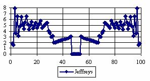
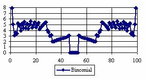
Figure 5. The percentages of the experimental errors for posttest probability

 at n = 100 (0 < X < n)

 

The percentages of the experimental errors for a sample size of 300 using specified method are in figure 6.

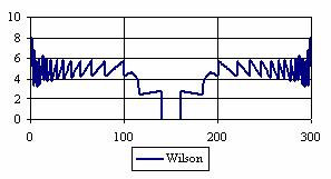
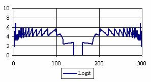
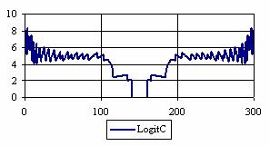
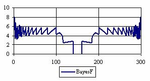
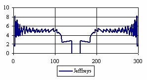
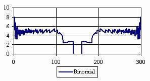
Figure 6. The percentages of the experimental errors

for posttest probability at n = 300 (0 < X < n)

 

The averages and standard deviations (into parenthesis) of experimental errors according to the sample size (n) and method used are in table 1.

 

Table 1. The averages of the experimental errors and standard deviations (parenthesis) for posttest probability at n = 10, 50, 100, 300 and 1000

 

The averages (MErr) and standard deviations (StdDev) of the experimental errors when n varies from 4 to 103 were presented in table 2.

 

 

Table 2. The average of the experimental errors and standard deviations

for posttest probability at 4 ≤  n < 104

 

Using the function (3) presented in materials and methods section of the paper, the graphical representation of frequencies of the best deviations relative to the imposed significance level (α = 5%) from figure 8 was obtained for 4 ≤  n < 104.

 

Figure 8. The frequencies of the best deviations of the experimental errors relative to significance level (α = 5%) for posttest probability at 4 ≤  n < 104

 

The contour plots of experimental errors when 4 ≤  n < 104 were illustrated in figure 7. On the plots were represented the experimental errors from 0% (red color) to 5% (yellow color) and ≥10% (blue color) using 18 intermediate hue. The vertical axis represent the n values (4 ≤  n < 104) and the horizontal axis the X values (from 0 to n-1).

Figure 7.  The contour plot of the experimental errors for ci3 function at 3 < n < 104

 

Figure 7.  The contour plot of the experimental errors for ci3 function at 3 < n < 104

 

Figure 7. The contour plot of the experimental errors for ci3 function at 3 < n < 104

 

The results of the deviations relative to the imposed significance level for 104 ≤ n ≤ 109 are in table 3.

 

Table 3. The deviations relative to the significance level (α = 5%)

for ci3 function at 104 ≤ n ≤ 109

 

For the random values of binomial variable (X) and sample sizes (n), when the random sample size is choused from 4 to 1000, a set of calculation were performed and graphical represented in figure 10.

In the figure 10 was represents with black dots the frequencies of the experimental error for each specified method; with green line the best errors interpolation curve with a Gauss curve (dIG(er)). The Gauss curves of the average and standard deviation of the experimental errors (dMV(er)) was represents with red line. The Gauss curve of the experimental errors deviations relative to the significance level (d5V(er)) was represented with blue squares. The Gauss curve of the standard binomial distribution from the average of the errors equal with 100·α (pN(er,10)) was represented with black line.

For the random samples, the results are in tables 4 to 7. In table 4 were presented the average of the deviation of the experimental errors relative to significance level α =5% (Dev5), the absolute differences of the average of experimental errors relative to the imposed significance level (|5-M|), and standard deviations (StdDev).

 

Table 4.  Methods ordered by performance according to Dev5, |5-M| and StdDev criterions

 

Table 5 contains the absolute differences of the averages that result from Gaussian interpolation curve to the imposed significance level (|5-MInt|), the deviations that result from Gaussian interpolation curve (DevInt), the correlation coefficient of interpolation (r2Int) and the Fisher point estimator (FInt).

Table 5. The methods ordered by |5-Mint|, DevInt, r2Int and FInt criterions

 

The superposition of the standard binomial distribution curve and interpolation curve (pNIG), the superposition of standard binomial distribution curve and the experimental error distribution curve (pNMV), and the superposition of standard binomial distribution curve and the error distribution curve around significance level (α = 5%) (pN5V) were presented in table 6.

 

Table 6. The confidence intervals methods ordered by the

pIGMV, pIG5V, and pMV5V criterions

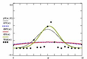
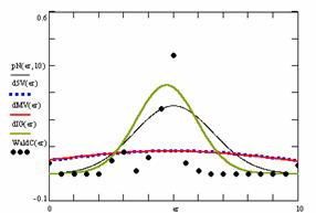
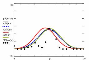
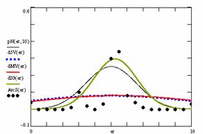
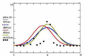
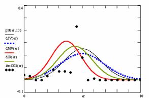
Figure 9. The pN(er, 10), d5V(er), dMV(er), dIG(er) and the frequencies of the experimental errors for each specified method for random X, n (1 ≤  X < 1000, 4 ≤ n ≤ 1000)

 

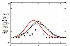
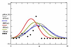
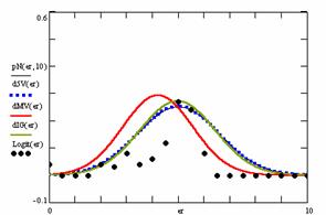
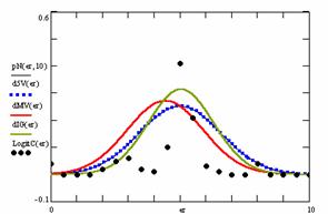
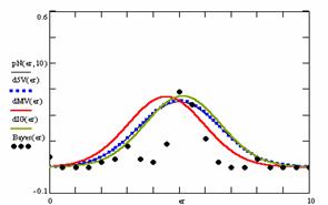
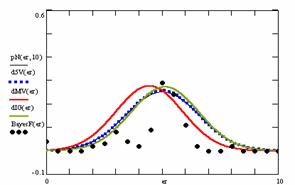
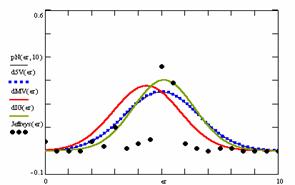
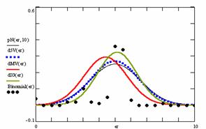
Figure 9. The pN(er, 10), d5V(er), dMV(er), dIG(er) and the frequencies of the experimental errors for each specified method for random X, n (1 ≤ X < 1000, 4 ≤ n ≤ 1000)

 

Table 7 contains the superposition of interpolation Gauss curve and the Gauss curve of error around experimental mean (pIGMV); the interpolation Gauss curve and the Gauss curve of error around imposed mean (pIG5V); and the  Gauss curve of experimental error around experimental mean and the error Gauss curve around imposed mean α = 5% (pMV5V).

 

Table 7. The confidence intervals ordered by the pIGMV, pIG5V, and pMV5V

 

 

Discussions

 

Analyzing the confidence intervals for posttest probability we can observe that for all methods of computing confidence intervals, the average of the experimental errors increases proportional with the increasing of the sample size and never exceeded the significance level (α = 5%).

The Logit and Jeffreys methods (both methods based on binomial distribution probability) obtains the most conservative experimental standard deviation in computing confidence intervals at a choused significance level equal with α = 5%. Thus, if we look after a confidence interval method, which is capable to assure the lowest standard deviation of the errors, we will choose one of these two methods.

If the standard deviation is not the ones parameter of confidence intervals assessment and we need a method which to assures an experimental error mean close to the significance level (α = 5%), then the LogitC method could be choused because obtain the best performance on the 100 ≤ n ≤ 300 domain. Even for n > 300, the best performance were obtain by the Logit (average of experimental errors equal with 4.53% at n=1000) followed by the BayesF (average of experimental errors equal with 4.50% at n=1000).

If we looked at the experimental results presented in table 2, according to different sample sizes, the methods Bayes, Binomial and Wilson obtains an average of the experimental errors closed to the choused significance level (α = 5%) and the Binomial method obtains the lowest standard deviation of the experimental errors.

Deviation relative to the imposed significance level (α = 5%) is a quantitative measure of performance of methods used in computing confidence intervals. Analyzing the figure 9 some aspects were disclosure. The first observation was that the original method Binomial improves the BayesF and the Jeffreys methods even if, the limit the Binomial overlap on BayesF and Jeffreys (see the Binomial function):

,

            The second observation is that from the binomial methods, the Binomial method obtains the best performance (with 70 appearances, followed by Jeffreys with 25 and the BayesF with 7 appearances).

            The third observation from the experimental data (which cannot been seen from the graphical plots) was that for n > 36 the Binomial method is almost systematically the method which have the lowest standard deviation, and it obtain one failure at n = 41 where the Jeffreys method obtains the lowest standard deviation. Note that from n ≥ 42, the Binomial method obtains the best performance in confidence intervals estimation for X/(2X-n) fraction.

For the random samples (n) and binomial variable (X), the WaldC method obtains the closed experimental error average to the significance level (see table 4); the lowest experimental standard deviation were obtains by the Clopper-Pearson method followed by the WilsonC method. The most closed deviation relative to the imposed significance level (α = 5%) was obtains by the Binomial method followed by the BayesF and Wilson methods.

The Logit method obtains the less absolute differences of the averages that results from the Gaussian interpolation curve to the imposed significance level (table 5), followed by the LogitC method; WaldC was the method with the lowest interpolation standard deviation. The Logit and the Agresti-Coull methods obtained the best correlation between theoretical curve and experimental data.

Analyzing the    results presented in the table 6, it can be observes that the Logit, BayesF and Agresti-Coull methods, obtain the maximum superposition of the interpolation curve and the curve of standard binomial distribution. The maximum superposition between the curve of standard binomial distribution and the curve of experimental errors was obtains by the Bayes method. The Logit and LogitC methods obtain the maximum superposition between the curve of standard binomial distribution and the curve of errors around the significance level (α = 5%).

The maximum superposition between the Gauss curve of interpolation and the Gauss curve of errors around experimental mean was obtains by the Bayes method, followed by the BayesF, LogitC and the Wilson methods (table 7).

The Logit method obtained the maximum superposition between the Gauss curve if interpolation and the Gauss curve of errors around significance level (α = 5%), followed by the method BayesF and the method Wilson. The maximum superposition between the Gauss curve of experimental errors and the Gauss curve of errors around imposed mean (α = 5%) were obtained by the Bayes method closely followed by the Wilson, LogitC and the BayesF methods.

 

 

Conclusions

 

The best criterion of comparing the methods of computing confidence intervals is deviation relative to the imposed significance level because in real experiments the sample sizes are not equal to each other.

The original Binomial method, systematically obtains the best performance for sample sizes of 36 ≤ n ≤ 1001, method that could be choused if it is need a method with the lowest standard deviation of the experimental errors.

The same performances are seen when the sample size vary from 4 to 103, where the Binomial method obtain the lowest deviations and also when the sample size and the binomial variable are randomly choused.

Based on these conclusions, we recommend the use of Binomial method for computing of the confidence intervals of posttest probability.

 

 

Acknowledgements

 

The first author is thankful for useful suggestions and all software implementation to Ph. D. Sci., M. Sc. Eng. Lorentz JÄNTSCHI from Technical University of Cluj-Napoca.

 

 

References