Binomial Distribution Sample Confidence Intervals Estimation
5. Odds Ratio
Sorana BOLBOACĂ, Andrei ACHIMAŞ CADARIU
“Iuliu Haţieganu” University of Medicine and Pharmacy, Cluj-Napoca, Romania
Abstract
Evaluation of the strength of association between predisposing or causal factors and disease can be express as odds ratio in case-control studies. In order to interpret correctly a point estimation of odds ratio we need to look also to its confidence intervals quality. The aim of this paper is to introduce three new methods of computing the confidence intervals, R2AC, R2Binomial, and R2BinomialC, and compare the performances with the asymptotic method called R2Wald.
In order to assess the methods a PHP program was develop. First, the upper and lower confidence boundaries for all implemented methods were computes and graphically represented. Second, the experimental errors, standard deviations of the experimental errors and deviation relative to the imposed significance level α = 5% were assessed. Estimating the experimental errors and standard deviations at central point for given sample sizes was the third criterion. The R2Wald and R2AC methods were assessed using random binomial variables (X, Y) and sample sizes (m, n) from 4 to 1000.
The methods based on the original method Binomial adjusted for odds ratio (R2Binomial, R2BinomialC functions) obtain systematically the lowest deviation of the experimental errors percent relative to the expected error percent and the R2AC method, the closest average of the experimental errors percent to the expected error percent.
Keywords
Confidence intervals estimation; Odds ratio; Case-control studies; Assessment of risk factors
Introduction
In medical studies if we look at the association between predisposing or causal factors and disease, the evaluation of the strength of the association can be express as the odds ratio in case-control studies or as the relative risk in cohort studies. In order to define the odds ratio, first we define the odds: "The concept of odds is similar to that of probability. The odds of having a disease are equal to the probability of contacting the disease divided by the probability of not contacting the disease". "The odds ratio compares the odds that exposed and nonexposed individual will have the disease, given by the relation: odds that exposed individual will have disease/odds that nonexposed individual will have the disease" [1]. Confidence intervals accompanying of odds ratio allowed a correct interpretations of the point estimation.
The Woolf procedure [2] describe the steps necessary to obtain the confidence intervals for the odds ratio, methods which was used in our experiment under the R2Wald name.
In the literature there we can find a series of article about the confidence intervals for odds ratio but all the methods were based on the Woolf procedure [3], [4]. AGRESTI Allan proposed a correction of the well-known confidence intervals asymptotic formula (Woolf method, named here R2Wald) [5] replacing the z1-α/2 with 2.
The aim of this paper is to introduce three new methods of computing the confidence intervals, represented by R2AC, R2Binomial and R2BinomialC, and comparing theirs, performances with the asymptotic method name R2Wald.
Materials and Methods
In medical studies of evaluation of a risk factors, when most of the time we have dichotomous variables the results can be organize in a 2 by 2 contingency table where four groups of cases can be define. First group is represent by the patients with diseases which are expose to the investigate risk factor (real positive cases), noted usually with a. Second group is represent by patients which do not present the disease but are expose to the investigate risk factor (false positive cases) usually noted with b.
Third group, the patients which present the disease but are not expose to the risk factor (false negative cases), usually noted with c and the fourth group, the patient which do not present the disease and not expose to the risk factor (true negative cases) usually noted with d.
Using the definition of the odds ratio and the next substitution on square two contingency table: a = X, b = Y, c = m-X, d = n-Y (X and Y are independent binomial distribution variables of sizes m and n) the odds ratio become:
![]() (1)
(1)
Thus, we can say that from mathematical point of view the odds ratio parameter is of X(n-Y)/Y/(m-X) function type, function named ci4 in our program [6].
Based on the classical definition of confidence intervals [7] and on our experiences in confidence intervals estimation, we defined four functions called R2Wald, R2AC, R2Binomial, and R2BinomailC:
 (2)
(2)
 (3)
(3)
 (4)
(4)
 (5)
(5)
where R2 function is computes by the formula (see also ref. [6]):
![]() (6)
(6)
The R2Wald is the standard method used in medical studies, known
as Woolf procedure. R2AC and R2Binomial methods are new
implemented methods. The R2AC method was obtained by introducing an
adjustment parameter represented by the ![]() parameter for the binomial variables (X,
Y) and
parameter for the binomial variables (X,
Y) and ![]() for
sample sizes (m, n), adjustment introduce by the Agresti and Coull to
the one-dimensional confidence intervals expression (CI = CI(X,n)) [8].
The R2Binomial method is base on the original method, Binomial,
method used for the first time in confidence intervals estimation of a
proportion [8].
for
sample sizes (m, n), adjustment introduce by the Agresti and Coull to
the one-dimensional confidence intervals expression (CI = CI(X,n)) [8].
The R2Binomial method is base on the original method, Binomial,
method used for the first time in confidence intervals estimation of a
proportion [8].
The above-described functions were implements into a PHP program. The PHP source codes for the functions are:
function R2Wald($X,$m,$Y,$n,$z,$a){
if($m-$X) $t1=1/($m-$X); else return array( 0 , (float)"INF" );
if($Y) $t4=1/$Y; else return array( 0 , (float)"INF" );
if((!$X)&&(!($n-$Y))) return array( 0 , pow($a/2,1/$m) * pow($a/2,1/$n) );
if($X) $t2=1/$X; return array( 0 , pow($a/2,1/$m)*$Y );
if($n-$Y) $t3=1/($n-$Y); else return array( 0 , pow($a/2,1/$n)*($m-$X) );
$t5=pow($t1+$t2+$t3+$t4,0.5)*$z;
return array( $X*($n-$Y)*exp(-$t5)/$Y/($m-$X) , $X*($n-$Y)*exp($t5)/$Y/($m-$X));}
function R2AC($X,$m,$Y,$n,$z,$a){
if($m==$X) return array( 0 , (float)"INF" ); if($Y==0) return array( 0 , (float)"INF" );
$ci = R2Wald($X+pow($z,2)/4/sqrt(2),$m+pow($z,2)/2/sqrt(2),
$Y+pow($z,2)/4/sqrt(2),$n+pow($z,2)/2/sqrt(2),$z,$a);
return array( $ci[0] , $ci[1] );}
function R2Binomial($X,$m,$Y,$n,$z,$a){
$ciX = Rap("Binomial",$X,$m,$z,sqrt($a/2));
$cinY = Rap("Binomial",$n-$Y,$n,$z,sqrt($a/2));
return array ( $ciX[0]*$cinY[0] , $ciX[1]*$cinY[1] );}
function R2BinomialC($X,$m,$Y,$n,$z,$a){
$ciX = Rap("Binomial",$X,$m,$z,(1/(1-0.125/log($m)))*sqrt($a/2));
$cinY = Rap("Binomial",$n-$Y,$n,$z,(1/(1-0.125/log($n)))*sqrt($a/2));
return array ( $ciX[0]*$cinY[0] , $ciX[1]*$cinY[1] );}
In order to obtain a 100·(1-α) = 95% confidence intervals (is most frequently used confidence intervals) the experiments were runs at a significance level α = 5% (noted with a in our program). Corresponding to choused significance level was used its normal distribution percentile z1-α/2 = 1.96 (noted with z in our program). The sequence of the program is:
define("z",1.96); define("a",0.05);
The performance of each method for different sample sizes (m, n) and different values of binomial variables (X, Y) was compares using a set of criterions.
First were computed and graphical represented the lower and upper confidence intervals limits for equal sample sizes (m = n = 50) using the R2BinomialC method:
$c_i=array("R2BinomialC");
define("N_min",50); define("N_max",51); est_ci2_er(z,a,$c_i, "ci4","ci");
Second, were analyzed the experimental errors and standard deviations of the experimental errors using the binomial distribution hypothesis as quantitative and qualitative criterion of the assessment and equal sample sizes (m = n = 5, 10, 20, and 40):
$c_i=array("R2Wald","R2AC","R2Binomial","R2BinomialC");
· For m = n = 5:
define("N_min",5); define("N_max",6); est_ci2_er(z,a,$c_i,"ci4","er");
· For m = n = 10 was modified:
define("N_min",10); define("N_max",11);
· For m = n = 20 was modified:
define("N_min",20); define("N_max",21);
· For m = n = 40 was modified:
define("N_min",40); define("N_max",41);
The standard deviation of the experimental error (StdDev) was computed using the next formula:
 (7)
(7)
where StdDev(X) is standard deviation, Xi is the experimental errors for a given i, M(X) is the arithmetic mean of the experimental errors and n is the sample size.
If we have a sample of n elements with a known (or expected) mean (equal with 100α), the deviation around α = 5% (imposed significance level) is giving by:
 (8)
(8)
Third, the assessment of the confidence intervals methods was carried on with a particular situation, represented by estimation of the experimental errors at central point (X = Y) and equals sample sizes m = n = 4, 6, 8..200 (m = n = even numbers):
$c_i=array("R2Wald","R2AC","R2Binomial","R2BinomialC");
define("N_min", 2); define("N_max",205); est_C2(z,a,$c_i,"ci4");
Fourth, the average of the experimental errors, standard deviation and deviation relative to the imposed significance level (α = 5%) were compute for sample sizes which vary from 4 to 14 (m=4..14, n = 4..14):
$c_i=array("R2Wald","R2AC","R2Binomial","R2BinomialC");
define("N_min", 4); define("N_max",15); est_C2(z,a,$c_i,"ci4", "mv");
The last part of the experiment consisted on assessing the performance of methods in 100 random numbers for binomial variables X, Y (4 ≤ X < n, 4 ≤ Y < m) and random sample sizes m, n ( 4 ≤ m, n ≤ 1000):
$c_i=array("R2Wald","R2AC");
define("N_min", 4); define("N_max",1000); est_ci2_er(z,a,$c_i,"ci4","ra");
The R2Binomial and R2BinomialC methods were not included in this part of the experiment because we did not have the resources needed to perform the experiment for the methods which used the hypothesis of binomial distribution.
Results
The confidence boundaries for odds ratio were computes, the results imported in SlideWrite Plus program (figure 1), and Microsoft Excel (figure 2) where the graphical representations were create.
The Slide representations (figure 1) were created using a 3D-Mesh graph type with 80% perspective, 60° tilt angle, and 75° rotation angle. On X-axis were represented the values of variable X, on the Y-axis the values Y variable and on the Z-axis were represented the odds ratio, lower or upper confidence intervals limits. There were represented with red color the experimental values from 0 to 2, with green the values from 2 to 4, with blue the values from 4 to 6, with cyan the values from 6 to 8, and with magenta the values from 8 to 10.
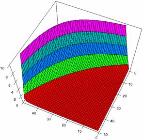
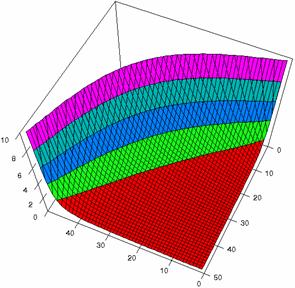
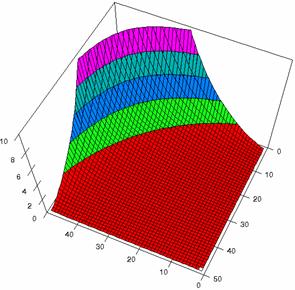
Figure2. The representation of the odds ratio values and its confidence limits obtained with R2BinomialC method at 0 < X, Y < m = n = 50
The lower and upper confidence limits in logarithmical scale with R2BinomialC method at equal sample sizes (m = n = 50) were graphical represented in figure 2. On horizontal axis were represented the m = n values (logarithmical scale), depending on X, Y and on the vertical axis the values of the confidence intervals limits (logarithmical scale).
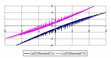
Figure 2. The upper and lower confidence limits (logarithmical scale) for odds ratio
at 0 < X, Y < m = n = 50
The contour plots of percentages of the experimental errors are in figure 3-6. On X-axis were represented the values of X binomial variable, on Y-axis the values of Y binomial variable, and on Z-axis the values of the percentage of experimental errors for each specified method. The graphical representations were created using a 3D-Mesh graph type with 80% perspective, 60° tilt angle and 75° rotation angle. On the plots were represented the percentages of the experimental errors with red color (0-2%), green (2-4%), blue (4-6%), cyan (6-8%), and magenta (8-10%).
The graphical representations of the percentages of the experimental errors using specified method for m = n = 5 were presented in figure 3; for m = n = 10 in figure 4; for m = n = 20 in figure 5; and for m = n = 40 in figure 6.
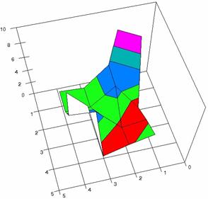
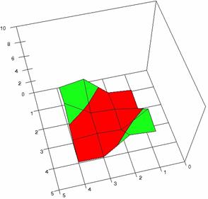
Figure 3. The OR experimental errors with R2Wald, and R2AC at 0<X,Y<m=n=5
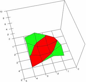
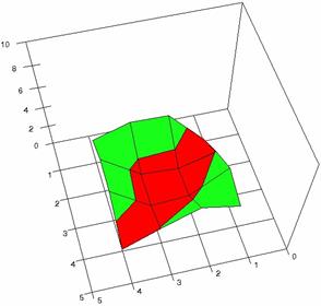
Figure 3. The OR experimental errors with R2Binomial, and R2BinomialC at 0<X,Y<m=n=5
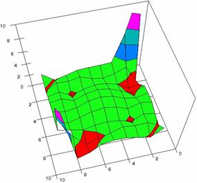
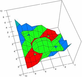
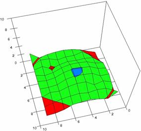
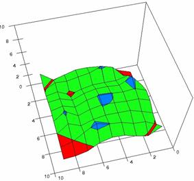
Figure 4. The OR experimental errors with R2Wald, R2AC R2Binomial, and R2BinomialC at 0 < X, Y < m = n = 10
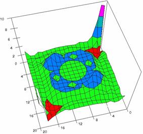
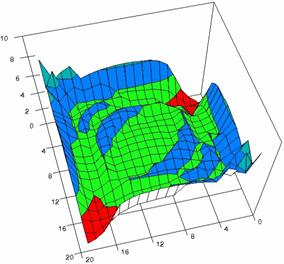
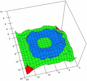
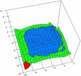
Figure 5. The OR experimental errors with R2Wald, R2AC, R2Binomial, and R2BinomialC
at 0 < X, Y < m = n = 20
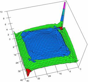
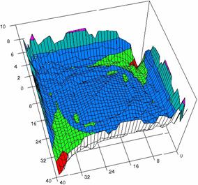
Figure 6. The OR experimental errors with R2Wald and R2AC at 0 < X, Y < m = n = 40
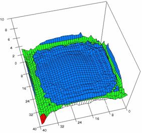
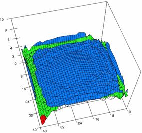
Figure 6. The OR experimental errors, R2Binomial and R2BinomialC at 0<X,Y<m=n=40
The averages (MErr) and standard deviations (StdDev) of the experimental errors for specified equal (m = n) samples sizes were presented in table 1.
|
n |
R2Wald |
R2AC |
R2Binomial |
R2BinomialC |
|
5 |
5.0 (6.1) |
1.7 (1.5) |
2.1 (1.2) |
2.3 (1.4) |
|
10 |
2.9 (2.0) |
3.1 (1.6) |
2.6 (0.8) |
2.9 (1.0) |
|
20 |
3.3 (1.2) |
3.9 (1.4) |
3.5 (1.0) |
3.9 (1.1) |
|
40 |
3.9 (1.0) |
4.5 (1.2) |
4.3 (0.8) |
4.5 (0.6) |
Table 1. The MErr and StdDev (parentheses) for odds ratio at m = n = 5, 10, 20, and 40
The confidence intervals for central point (X = Y) were calculated and the graphical representations was creates (figure 7). In the graphical representation, on horizontal axis were represented the values of samples sizes (m = n = 4,6..200 (even numbers)) depending on X = Y values; on the vertical axis were represented the percentage of the experimental errors.
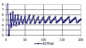
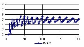
Figure 7. The percentages of the experimental errors for odds ratio at central point X = Y
and at m= n = 4,6,..200
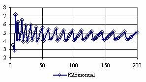
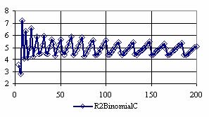
Figure 7. The percentages of the experimental errors for odds ratio at central point X = Y
and at m= n = 4,6,..200
The average of the percentages of experimental errors (MErr) and the standard deviations (StdDev) of them for central point estimation (X = Y) are in table 2.
|
Method |
R2Wald |
R2AC |
R2Binomial |
R2BinomialC |
|
MErr |
4.91 |
4.60 |
4.69 |
4.89 |
|
StdDev |
0.76 |
0.81 |
0.62 |
0.60 |
Table 2. The MErr and StdDev for OR at central point (X=Y) and m = n = 4,6..200
The surface plots of dependences of averages of the experimental errors (left side) and of the deviations relative to the imposed significance level α = 5% (right side) for sample sizes varying in the range 4..14 were graphically represented in figure 8.
The dependency surface plots were created with 80% perspective, 40° tilt angle and 45° rotation angle (for experimental errors average) and with 15° rotation angle (for standard deviations). For the graphical representation of averages of the experimental errors (left side graphics), with red color were represented the experimental values from 0 to 2, with green the values from 2 to 4, with blue the values from 4 to 6, with cyan the values from 6 to 8, and with magenta the values from 8 to 10.
In the graphical representation of dependency of the deviations relative to the significance level (α = 5%) (right side), with red color were represented the experimental values from 2 to 2.5, with green color the values from 2.5 to 3, with blue the values from 3 to 3.5, with cyan the values from 3.5 to 4, with magenta the values from 4 to 4.5, and with yellow the values from 4.5 to 5.
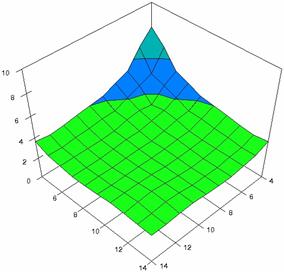
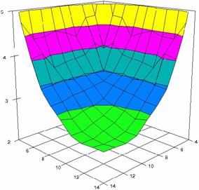
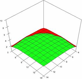
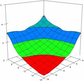
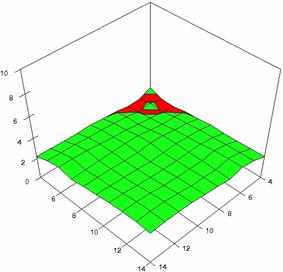
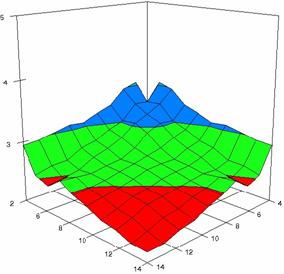
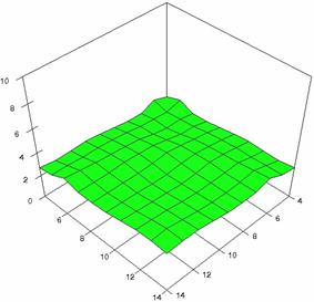
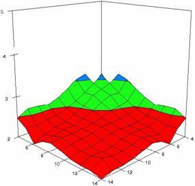
Figure 8. Dependences of the averages of experimental errors and of deviations relative to imposed significance level for OR with R2BinomialC at m, n = 4..14
The averages of the means of experimental errors (MMErr) and of the deviations relative to the imposed significant level α = 5% (MDev5) for sample sizes which vary in 4..14 domain are in table 3.
|
Method |
R2Wald |
R2AC |
R2Binomial |
R2BinomialC |
|
MMErr |
3.33 |
2.64 |
2.57 |
2.95 |
|
MDev5 |
3.90 |
2.92 |
2.70 |
2.41 |
Table 3. The averages and deviations relative to α = 5% of experimental errors for OR when sample size m, n vary in 4..14 domain
Using the results obtained from the 100 random binomial variable (X, Y; 0 < X, Y < m, n) and samples size (n, m) from 4 to 1000 domain (4 ≤ m, n ≤ 1000), a set of calculations as are described in paper [6] are done and presented in tables 4-7 and represented in figure 9.
In the figure 9 were represented with black dots the frequencies of the experimental error for each specified method; with green line the best errors interpolation curve with a Gauss curve (dIG(er)). The Gauss curves of the average and standard deviation of the experimental errors (dMV(er)) was represents with red line. The Gauss curve of the experimental errors deviations relative to the significance level (d5V(er)) was represented with blue squares. The Gauss curve of the standard binomial distribution from the average of the errors equal with 100·α (pN(er,10)) was represented with black line.
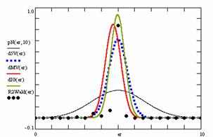
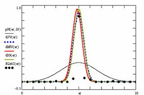
Figure 9. The pN(er, 10), d5V(er), dMV(er), dIG(er) and the frequencies of the experimental errors for each specified method and random X, m, Y, n (0 < X, Y < m, n; 4 ≤ m, n ≤ 1000)
Table 4 contain the average of the deviation of the experimental errors relative to significance level α = 5% (Dev5), the absolute differences of the average of experimental errors relative to the imposed significance level (|5-M|), and standard deviations (StdDev).
|
No |
Method |
Dev5 |
Method |
|5-M| |
Method |
StdDev |
|
1 |
R2AC |
0.44 |
R2AC |
0.13 |
R2AC |
0.42 |
|
2 |
R2Wald |
0.56 |
R2Wald |
0.29 |
R2Wald |
0.47 |
Table 4. Methods ordered by performance according to Dev5, |5-M| and StdDev criterions
Table 5 contains the absolute differences of the averages that result from Gaussian interpolation curve to the imposed significance level (|5-MInt|), the deviations that result from Gaussian interpolation curve (DevInt), the correlation coefficient of interpolation (r2Int) and the Fisher point estimator (FInt).
|
No |
Method |
|5-MInt| |
Method |
DevInt |
Method |
r2Int |
FInt |
|
1 |
R2AC |
0.00 |
R2AC |
0.42 |
R2Wald |
0.76 |
60 |
|
2 |
R2Wald |
0.02 |
R2Wald |
0.43 |
R2AC |
0.77 |
62 |
Table 5. The methods ordered by |5-MInt|, DevInt, r2Int and FInt criterions
The superposition of the standard binomial distribution curve and interpolation curve (pNIG), the superposition of standard binomial distribution curve and the experimental error distribution curve (pNMV), and the superposition of standard binomial distribution curve and the error distribution curve around significance level (α = 5%) (pN5V) were presented in table 6.
|
No |
Method |
pNIG |
Method |
pNMV |
Method |
pN5V |
|
1 |
R2AC |
0.44 |
R2AC |
0.44 |
R2AC |
0.45 |
|
2 |
R2Wald |
0.44 |
R2Wald |
0.47 |
R2Wald |
0.54 |
Table 6. Methods ordered by the pNIG, pNMV, and pN5V criterions
In table 7 were presented the percentages of superposition of the interpolation Gauss curve and of the Gauss curve of error around experimental mean (pIGMV), between the interpolation Gauss curve and the Gauss curve of error around imposed mean (α = 5%) (pIG5V), and between the Gauss curve experimental error around experimental mean and the error Gauss curve around imposed mean α = 5% (pMV5V).
|
No |
Method |
pIGMV |
Method |
pIG5V |
Method |
pMV5V |
|
1 |
R2AC |
0.87 |
R2AC |
0.98 |
R2AC |
0.88 |
|
2 |
R2Wald |
0.76 |
R2Wald |
0.87 |
R2Wald |
0.77 |
Table 7. The confidence intervals ordered by the pIGMV, pIG5V, and pMV5V criterions
Discussions
For the equal sample sizes, if we look after a method which to obtained an average of the experimental error closest to the imposed significance level (α = 5%), the R2Wald method can be chouse if m = n = 5. On the other hand, the R2Wald method obtained the greatest standard deviation compared with the R2AC, R2Binomial, and R2BinomialC methods. The best standard deviation for m = n = 5 was obtains by the R2Binomial. For the R2AC, R2Binomial and R2BinomialC methods the averages of the experimental errors increase with sample sizes but never exceed the significance level (α = 5%). The best performance in confidence intervals estimation for m = n = 40, as well as for m = n = 20, is obtain by the R2BinomialC and the R2AC methods.
The best average of the experimental errors for central point (X=Y) was obtained by the asymptotic method (R2Wald) and the best performance at the central point was obtained with a binomial method (R2BinomialC, closely followed by the R2Binomial method).
If we looked at the special experiment when sample sizes vary in 4..14 domain, for all methods, the averages of experimental errors were less than the expected value (α = 5%); the R2Wald method was the one which obtained the greatest average of the errors (3.33%). The lowest standard deviation was obtains by the R2Binomial method.
Looking at the results from random binomial variables (X, Y) and random samples (m, n) we can remarked that the R2AC method obtains the closest experimental error average to the significance levels (table 4), the lowest experimental standard deviation and the closest deviation of the experimental errors to the significance level (α = 5%).
The R2AC method obtains the closest interpolation average to the significance level (table 5), the lowest interpolation deviation, and the best correlation between theoretical curve and experimental data.
The R2Wald method (as well as the R2AC method) obtains the maximum superposition between the curve of interpolation and the curve of standard binomial distribution, the maximum superposition between the curve of standard binomial distribution and the curve of experimental errors. Again the R2Wald method obtained the maximum superposition between the curve of standard binomial distribution and the curve of error distribution around the significance level (α = 5%).
The maximum superposition between the Gauss curve of interpolation and the Gauss curve of errors around experimental mean obtains by the R2AC method. The R2AC method obtained again the maximum superposition between the Gauss curve of interpolation and the Gauss curve of errors around significance level (α = 5%), and the maximum superposition between the Gauss curve of experimental errors and the Gauss curve of errors around imposed mean (α = 5%).
Acknowledgements
The first author is thankful for useful suggestions and all software implementation to Ph. D. Sci., M. Sc. Eng. Lorentz JÄNTSCHI from Technical University of Cluj-Napoca.
References