A Genetic Algorithm for Solving the Optimal Power Flow Problem

Tarek BOUKTIR^a, Linda SLIMANI^a, M. BELKACEMI^b

^a Department of Electrical Engineering, University of Oum El Bouaghi,04000, Algeria. Email:tbouktir@lycos.com; Tel/Fax: (213) 32 42 23 85 or (213) 32 42 10 36

^b Department of Electrical Engineering, University of Batna, Algeria Email: Belkacemi_M@hotmail.com

Abstract

This paper presents solution of optimal power flow problem of large distribution systems via a simple genetic algorithm. The objective is to minimize the fuel cost and keep the power outputs of generators, bus voltages, shunt capacitors/reactors and transformers tap-setting in their secure limits. CPU times can be reduced by decomposing the optimization constraints to active constraints manipulated directly by the genetic algorithm, and passive constraints maintained in their soft limits using a conventional constraint load flow. The IEEE 30-bus system has been studied to show the effectiveness of the algorithm.

Keyworks

Load flow, optimal power flow, and genetic algorithm.

I. INTRODUCTION

The optimal power flow has been frequently solved using classical optimization methods. The OPF has been usually considered as the minimization of an objective function representing the generation cost and/or the transmission loss. The constraints involved are the physical laws governing the power generation-transmission systems and the operating limitations of the equipment.

Effective optimal power flow is limited by (i) the high dimensionality of power systems and (ii) the incomplete domain dependent knowledge of power system engineers. The first limitation is addressed by numerical optimization procedures based on successive linearization using the first and the second derivatives of objective functions and their constraints as the search directions or by linear programming solutions to imprecise models [1-4]. The advantages of such methods are in their mathematical underpinnings, but disadvantages exist also in the sensitivity to problem formulation, algorithm selection and usually converge to a local minimum [5]. The second limitation, incomplete domain knowledge, precludes also the reliable use of expert systems where rule completeness is not possible.

Genetic algorithms offer a new and powerful approach to these optimization problems made possible by the increasing availability of high performance computers at relatively low costs. These algorithms have recently found extensive applications in solving global optimization searching problems when the closed-form optimization technique cannot be applied. Genetic algorithms (GAs) are parallel and global search techniques that emulate natural genetic operators. The GA is more likely to converge toward the global solution because it, simultaneously, evaluates many points in the parameter space. It does not need to assume that the search space is differentiable or continuous [6] In recent paper [7], the Genetic Algorithm

Optimal Power Flow (GAOPF) problem is solved based on the use of a genetic algorithm load flow, and to accelerate the concepts it propose the use of gradient information by the use of the steepest decent method. The method is not sensitive to the starting points and capable to determining the global optimum solution to the OPF for range of constraints and objective functions. But GAOPF requires two load flow to be performed per individual, per iteration because all controllable variables are included in the fitness. In this paper we develop a simple genetic algorithm applied to the problem of optimal power flow in large power distribution systems. To accelerate the processes of GAOPF, the controllable variables are decomposed to active constraints that effect directly the cost function are included in the Genetic algorithms process and passive constraints which are updating using a conventional load flow program, only, one time after the convergence on the GAOPF. In which the search of the optimal parameters set is performed using into the account that the power losses are 2% of the power demand. The slack bus parameter would be recalculated in the load flow process to take the effect of the passive constraints.

II. PROBLEM FORMULATION

The standard OPF problem can be written in the following form,

Minimise F(x)                                                   (the objective function)

subject to :

hi(x) = 0, i = 1, 2, ..., n                                   (equality constraints)

gj(x) = 0, j = 1, 2, ...,m                                   (inequality constraints)

where x is the vector of the control variables, that is those which can be varied by a control center operator (generated active and reactive powers, generation bus voltage magnitudes, transformers taps etc.);

The essence of the optimal power flow problem resides in reducing the objective function and simultaneously satisfying the load flow equations (equality constraints) without violating the inequality constraints

A. Objective Function

The most commonly used objective in the OPF problem formulation is the minimisation of the total cost of real power generation. The individual costs of each generating unit are assumed to be function, only, of active power generation and are represented by quadratic curves of second order. The objective function for the entire power system can then be written as the sum of the quadratic cost model at each generator.

                                                                       (1)

where ng is the number of generation including the slack bus. Pgi is the generated active power at bus i. a_i, b_i and c_i are the unit costs curve for i^th generator.

B. Types of equality constraints

While minimizing the cost function, its necessary to make sure that the generation still supplies the load demands plus losses in transmission lines. Usually the power flow

equations are used as equality constraints.

                                                             (2)

where active and reactive power injection at bus i are defined in the following equation:

                                       (3)

C. Types of inequality constraints

The inequality constraints of the OPF reflect the limits on physical devices in the power system as well as the limits created to ensure system security. The most usual types of inequality constraints are upper bus voltage limits at generations and load buses, lower bus voltage limits at load buses, var. limits at generation buses, maximum active power limits corresponding to lower limits at some generators, maximum line loading limits and limits on tap setting of TCULs and phase shifter. The inequality constraints on the problem variables considered include:

• Upper and lower bounds on the active generations at generator buses P_gi^min ≤P_gi ≤ P_gi^max , i = 1, ng.

• Upper and lower bounds on the reactive power generations at generator buses and reactive power injection at buses with VAR compensation Q_gi^min ≤ Q_gi ≤ Q_gi^max, i = 1, npv

• Upper and lower bounds on the voltage magnitude at the all buses V_i^min ≤ V_i ≤ V_i^max , i = 1, nbus.

• Upper and lower bounds on the bus voltage phase angles: , i = 1, nbus.

It can be seen that the generalized objective function F is a non-linear, the number of the equality and inequality constraints increase with the size of the power distribution systems. Applications of a conventional optimization technique such as the gradient-based algorithms to a large power distribution system with a very non-linear objective functions and great number of constraints are not good enough to solve this problem. Because it depend on the existence of the first and the second derivatives of the objective function and on the well computing of these derivative in large search space.

III. GENETIC ALGORITHM IN OPTIMAL POWER FLOW

A. Description of Genetic Algorithms

The genetic algorithms are part of the evolutionary algorithms family, which are computational models, inspired in the Nature. Genetic algorithms are powerful stochastic search algorithms based on the mechanism of natural selection and natural genetics. GAs works with a population of binary string, searching many peaks in parallel. By employing genetic operators, they exchange information between the peaks, hence reducing the possibility of ending at a local optimum. GAs are more flexible than most search methods because they require only information concerning the quality of the solution produced by each parameter set (objective function values) and not lake many optimization methods which require derivative information, or worse yet, complete knowledge of the problem structure and parameters.

There are some difference between GAs and traditional searching algorithms [8][9]. They cold be summarized as follows:

• The algorithms work with a population of string, searching many peaks in parallel, as opposed to a single point.

• GAs work directly with strings of characters representing the parameters set not the parameters themselves.

• GAs use probabilistic transition rules instead of deterministic rules.

• GAs use objective function information instead of derivatives or others auxiliary knowledge.

• GAs have the potential to find solutions in many different areas of the search space simultaneously.

B. GA Applied to optimal power flow

A simple Genetic Algorithm is an iterative procedure, which maintains a constant size population P of candidate solutions. During each iteration step (generation) three genetic operators (reproduction, crossover, and mutation) are performing to generate new populations (offspring), and the chromosomes of the new populations are evaluated via the value of the fitness witch is related to cost function. Based on these genetic operators and the evaluations, the better new populations of candidate solution are formed.

With the above description, a simple genetic algorithm is given as follow [6]:

1. Generate randomly a population of binary string

2. Calculate the fitness for each string in the population

3. Create offspring strings through reproduction, crossover and mutation operation.

4. Evaluate the new strings and calculate the fitness for each string (chromosome).

5. If the search goal is achieved, or an allowable generation is attained, return the best chromosome as the solution; otherwise go to step 3.

We now describe the details in employing the simple GA to solve the optimal power flow problem.

B.1 Chromosome coding and decoding

GAs works with a population of binary string, not the parameters themselves. For simplicity and convenience, binary coding is used in this paper. With the binary coding method, the active generation power set of 9-bus test system (Pg1,Pg2 and Pg3) would be coded as binary string of O’s and 1’ with length B₁, B₂, and B₃ (may be different), respectively. Each parameter Pg_i have upper bound U_i and lower bound Li .The choice of B₁, B₂, and B₃ for the parameters is concerned with the resolution specified by the designer in the search space. In the binary coding method, the bit length B_i and the corresponding resolution

R_i is related by

                                                                                                    (4)

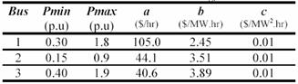
As result, the Pgi set can be transformed into a binary string (chromosome) with length ÓBi and then the search space is explored. Note that each chromosome present one possible solution to the problem. For example, suppose the parameter domain of (Pg₁,Pg₂ and Pg₃) which is presented in Table I:

TABLE I. PARAMETER SET OF Pg₁

If the resolution (R₁, R₂, R₃) is specified as (0.1, 0.05, 0.1), from (3) we have (B₁, B₂, B₃)=(4,4,4). Then the parameter set (Pg₁,Pg₂ and Pg₃) can be coded according to the following (Table II):

TABLE II. CODING OF Pg_i PARAMETER SET

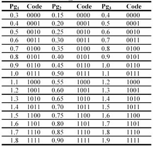
If the candidate parameters set is (1.7, 0.30, 1.1), then the chromosome is a binary string 111000110111. The decoding procedure is the reverse procedure.

The first step of any genetic algorithm is to generate the initial population. A binary string of length L is associated to each member (individual) of the population. The string is usually known as a chromosome and represents a solution of the problem. A sampling of this initial population creates an intermediate population. Thus, some operators (reproduction, crossover and mutation) are applied to this new intermediate population in order to obtain a new one.

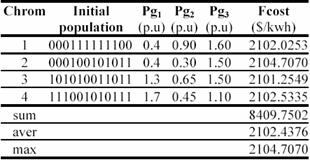
Process, that starts from the present population and leads to the new population, is named a generation when executing a genetic algorithm (Table III).

TABLE III. First generation of GA process for 9bus example

B.2 Crossover

Crossover is the primary genetic operator, which promotes the exploration of new regions in the search space. For a pair of parents selected from the population the recombination operation divides two strings of bits into segments by setting a crossover point at random, i.e. Single Point Crossover. The segments of bits from the parents behind the crossover point are exchanged with each other to generate their offspring. The mixture is performed by choosing a point of the strings randomly, and switching their segments to the left of this point. The new strings belong to the next generation of possible solutions. The strings to be crossed are selected according to their scores using the roulette wheel [6]. Thus, the strings with larger scores have more chances to be mixed with other strings because all the copies in the roulette have the same probability to be selected.

B.3 Mutation

Mutation is a secondary operator and prevents the premature stopping of the algorithm in a local solution. The mutation operator is defined by a random bit value change in a chosen string with a low probability of such change. The mutation adds a random search character to the genetic algorithm, and it is necessary to avoid that, after some generations, all possible solutions were very similar ones.

All strings and bits have the same probability of mutation. For example, in the string 110011101101, if the mutation affects to time bit number six, the string obtained is 110011001101 and the value of Pg₂ change from 0.85 p.u to 0.75 p.u.

B.4 Reproduction

Reproduction is based on the principle of survival of the better fitness. It is an operator that obtains a fixed number of copies of solutions according to their fitness value. If the score increases, then the number of copies increases too. A score value is of associated to a given solution according to its distance of the optimal solution (closer distances to the optimal solution mean higher scores).

B.5 Fitness of candidate solutions and cost function

The cost function is defined as:

                                     (5)

Our objective is to search (Pg₁,Pg₂,Pg₃) in their admissible limits to achieve the optimization problem of OPF. The cost function F(x) takes a chromosome (a possible (Pg₁,Pg₂,Pg₃) and returns a value. The value of the cost is then mapped into a fitness value Fit(Pg₁,Pg₂,Pg₃) so as to fit in the genetic algorithm.

To minimize F(x) is equivalent to getting a maximum fitness value in the searching process. A chromosome that has lower cost function should be assigned a larger fitness value.

The objective of OPF has to be changed to the maximization of fitness to be used in the simulated roulette wheel as follows:

                                                    (6)

Then the GA tries to generate better offspring to improve the fitness. Using the above components, a standard GA procedure for solving the optimal power flow problem is summarized in the diagram of the Figure 1.

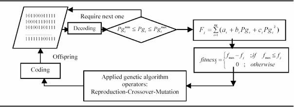
Figure 1.  A Simple flow chart of the GAOPF

The use of penalty functions in many OPF solutions techniques to handle generation bus reactive power limits can lead to convergence problem due to the distortion of the solution surface. In this method no penalty functions are required. Because only the active power of generators are used in the fitness. And the reactive levels are scheduled in the load flow process. Because his essence of this idea is that the constraints are partitioned in two types of constraints, active constraints are checked using the GA procedure and the reactive constraints are updating using an efficient Newton-Raphson Load flow procedure.

C. Load Flow calculation

After the search goal is achieved, or an allowable generation is attained by the genetic algorithm. It’s required to performing a load flow solution in order to make fine adjustments on the optimum values obtained from the GAOPF procedure. This will provide updated voltages, angles and transformer taps and points out generators having exceeded reactive limits. to determining all reactive power of all generators and to determine active power that it should be given by the slack generator using into account the deferent reactive constraints. Examples of reactive constraints are the min and the max reactive rate of the generators buses and the min and max of the voltage levels of all buses. All these require a fast and robust load flow program with best convergence properties.

The developed load flow process is based upon the full Newton-Raphson algorithm using the optimal multiplier technique [10][11].

IV. APPLICATION STUDY

The GAOPF has been developed by the use of Borland C++ Builder version 5. It is tested using the modified IEEE 30-bus system [12].The system consists of 41 lines, 6 generators, 4 Tap-changing transformers, and shunt capacitor banks located at 9 buses (Figure 2). The parameter settings to execute GAOPF are probability of crossover = 0.5, probability of mutation = 0.7, the population size is 48, the power mismatch tolerance is 0.0001 p.u and other parameters are presented in (Table IV).

TABLE IV. Power Generation Limits and Generator Cost Parameters of Ieee 30-Bus System In P.U (Sb=100mva)*

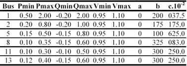
* In Table IV, Pmin, Pmax, Qmin, Qmax, Vmin and Vmax are in (p.u), a in ($/hr), b in ($/MW.hr) and c in (($/MW².hr).

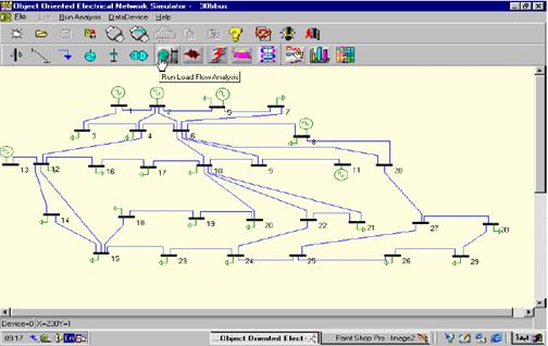
Figure 2. IEEE 30-bus electrical system topology

drawing by our OOENS software ver. 3.00 [13]

To compare these results with conventional method using the same cost objective function we have take conventional method present in [13]. The method is based on a Quasi-Newton Method using Broyden-Fletcher-Goldfarb-Shanno (BFGS) updating formula and iterated with the Newton Raphson load flow. The resulting cost and power losses are presented in (Table V).

The result show that the method presented gives much better results than the other method. The difference in generation cost between these two studies (803.699 $/kW∙hr compared to 807,782 $/kW∙hr) and in Real power loss (9.5177 MW compared to 8.805 MW) clearly shows the advantage of this method. In addition, it is important to point out that this simple genetic algorithm OPF converge in an acceptable time. For this test system was approximately 7 seconds, and it converged to highly optimal solutions set after 20 generations tested with Pentium I, 166 MHZ, 32MO. The optimum active power is in their secure values and is far from the min and max limits. It is also clear from the optimum solution that the GA easily prevent the violation of all the active constraints. The security constraints are also checked for voltage magnitudes and angles (Figure 3). The voltage magnitudes and the angles are between their minimum and the maximum values. No load bus was at the lower limit of the voltage magnitudes (0.9 p.u).

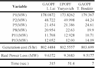
The proposed GAOPF is also compared with the evolutionary methods of references [7,8].

The published evolutionary method of Lai and al., is based on GA with the dynamic hierarchy of the coding system in order to be able to code a large number of control variables in a practical system within a reasonable length string.

The other one which is writing by Janson Yurevich and Kit Po Wong is an evolutionary programming with the inclusion of gradient information to speed the search in areas local to candidate solutions.

The results including the generation cost, real power losses and convergence time compared with published evolutionary methods are shown in Table VI.

The results are similar to those obtained with the published evolutionary programming based OPF program and using the same cost objective function. It is also important to point out that the computing time of this GAOPF compared with that of the published evolutionary methods is better by more than a 9:1 speed ratio.

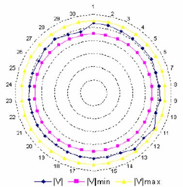
Fig.3 Voltage levels of IEEE 30 Bus electrical Network

TABLE V. Results of GAOPF Compared with Evolutionary

Methods for the IEEE 30-Bus System

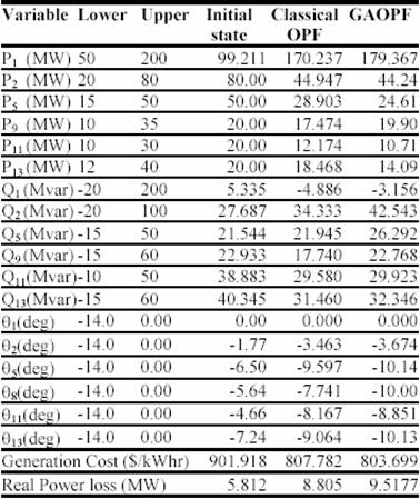
TABLE VI . Results of GAOPF Compared with Evolutionary Methods

V. CONCLUSION

Application of Genetic approach to Optimal Power Flow has been explored and tested. A simulation results show that a simple genetic algorithm can give a best result using only simple genetic operations such as proportionate reproduction, simple mutation, and one-point crossover in binary codes. It’s recommended to indicate that in large-scale system the number of constraints are very large consequently the GA accomplished in a large CPU time.

To save an important CPU time, the constraints are to be decomposing in active constraints and reactive ones. The active constraints are the parameters whose enter directly in

the cost function and the reactive constraints are infecting the cost function indirectly. With this approach, only the active constraints are taken to calculate the optimal solution set. And the reactive constraints are taking in an efficient load flow by recalculate active power of the slack bus. The developed system was then tested and validated on the IEEE30-bus system. Solutions obtained with the developed Genetic Algorithm Optimal Power Flow program has shown to be almost as fast as the solutions given by a conventional language. Our GAOPF appears to be faster than other published GAOPF methods.

REFERENCES

[1] H. W. Dommel, W. F. Tinney, Optimal Power Flow Solutions, IEEE Transactions on power apparatus and systems, Vol. PAS-87, No. 10, p. 1866-1876, October 1968.

[2] K. Y. Lee, Y.M. Park, and J.L. Ortiz, A United Approach to Optimal Real and Reactive Power Dispatch, IEEE Transactions on Power Systems, Vol. PAS-104, p. 1147-1153, May 1985.

[3] M. Sasson, Non linear Programming Solutions for load flow, minimum loss, and economic dispatching problems, IEEE Trans. on power apparatus and systems, Vol. PAS-88, No. 4, April 1969.

[4] T. Bouktir, M. Belkacemi, K. Zehar, Optimal power flow using modified gradient method, Proceeding ICEL’2000, U.S.T.Oran, Algeria, Vol. 2, p. 436-442, 13-15 November 2000.

[5] R. Fletcher, Practical Methods of Optimisation, John Willey & Sons, 1986.

[6] D. E. Goldberg Genetic Algorithms in Search, Optimization and Machine Learning, Addison Wesley Publishing Company, Ind. USA, 1989.

[7] J. Yuryevich, K. P. Wong, Evolutionary Programming Based Optimal Power Flow Algorithm, IEEE Transaction on power Systems, Vol. 14, No. 4, November 1999.

[8] L.L. Lai, J. T. Ma, R. Yokoma, M. Zhao Improved genetic algorithms for optimal power flow under both normal and contingent operation states, Electrical Power & Energy System, Vol. 19, No. 5, p. 287-292, 1997.

[9] B. S. Chen, Y. M. Cheng, C. H. Lee, A Genetic Approach to Mixed H2/H00 Optimal PID Control, IEEE Control system, p. 551-59, October 1995.

[10] Glenn W. Stagg, Ahmed H. El Abiad, Computer methods in power systems analysis, Mc Graw Hill international Book Campany, 1968.

[11] S. Kumar, R. Billinton, Low bus voltage and ill-conditioned network situation in a composite system adequacy evaluation, IEEE transactions on power systems, vol. PWRS-2, No. 3, August 1987.

[12] L. Terra, M. Short, Security constrained reactive power dispatch, IEEE transaction on power systems, Vol. 6, No. 1, February 1991.

[13] T. Bouktir , M. Belkacemi , L. Benfarhi and A. Gherbi, Oriented Object Optimal Power Flow, the UPEC 2000, 35^th Universities Power Engineering Conferences Belfast, Northern Ireland, 6-8 September 2000.