Binomial Distribution Sample Confidence Intervals Estimation
8. Number Needed to Treat/Harm
Sorana BOLBOACĂ, Andrei ACHIMAŞ CADARIU
Iuliu Haţieganu University of Medicine and Pharmacy, Cluj-Napoca, Romania
Abstract
Nowadays, the number needed to treat became the most important parameter in reporting the treatment effects in clinical trials, from binary outcomes such as positive or negative. Defined as a reciprocal of the absolute risk reduction, the number needed to treat is the number of patients who need to be treated to prevent one additional adverse even. In medical literature, the number needed to treat is reported usually with its asymptotic confidence intervals, method that is used by the most software packages even if it is knows that is not the best method. The aim of this paper is to introduce three new methods of computing confidence intervals for number needed to treat/harm.
Using PHP programming language was implementing the proposed methods and the asymptotic one (called here IADWald). The performance of each method, for different sample sizes (m, n) and different values of binomial variables (X, Y) were asses using a set of criterions: the upper and lower boundaries; the average and standard deviation of the experimental errors; the deviation of the experimental errors relative to imposed significance level (α = 5%). The methods were assess on random binomial variables X, Y (where X < m, Y < n) and random sample sizes m, n (4 ≤ m, n ≤ 1000).
The performances of the implemented methods of computing confidence intervals for number needed to treat/harm are present in order to be taking into consideration when a confidence interval for number needed to treat is used.
Keywords
Confidence intervals; Binomial distributions; Number needed to treat; Number needed to harm; Therapy studies assessment
Introduction
In therapy studies, treatment effects from binary outcomes, such as positive or negative, can be present in various ways (e.g., relative risk reduction, absolute risk reduction, number needed to treat) [1]. LAUPACIS et al introduced the concept of number needed to treat as an alternative approach to summarizing the effect of treatment [2]. The number needed to treat is defining as the number of patients who need to be treated to prevent one additional adverse even [3], [4]. When the experimental treatment increases the risk of an undesirable outcome/event the number needed to harm can be compute. The number needed to harm has the same mathematical expression as number needed to treat [1], [5].
Some journals provide today the point estimation of number needed to treat/harm along with its confidence intervals [6]. ATLMAN [6] recommend that the confidence intervals should always be gives when a number needed to treat/harm is reports as study result. The confidence limits for the number needed to treat are the inverse of the limits for the absolute risk reduction [3], [7]. Unfortunately the only method reported in medical literature for number needed to treat/harm is the asymptotic method (called here IADWald) which is well known that provide too short confidence intervals [6], [8], [9]. BENDER proposed a new method based on Wilson score, method that improves the calculation of confidence intervals for number needed to treat/harm [10].
The aim of this paper is to introduce three methods of computing the confidence intervals for number needed to treat/harm.
Materials and Methods
In medical studies where a treatment effects is measure as a binary outcomes, such as efficacious or non-efficacious, a 2´2 contingency table can be create. The table contains four groups of cases: real positive cases (patients which receive the new treatment and at which the treatment was efficacious) noted usually with a; false positive cases (patients which receive the new treatment and at which the treatment has no effect), noted usually with b. The false positive cases (patients which receive a placebo drug and at which the outcome of interest was present), noted usually with c, and the true negative cases (patients which receive a placebo drug and at which the outcome of interest was not present), noted usually with d.
According with the outcome of the experimental treatment, based on the same mathematical formula can be compute the number needed to treat (NNT) and the number needed to harm (NNH). Using following substitutions: a = Y, b = n-Y, c = X, d = m-X, where X and Y are independent binomial variables of sizes m and n, the number needed to treat becomes:
 (1)
(1)
From the mathematical point of view, the number needed to treat/harm is equals with the reciprocal of the absolute risk reduction (|1/(Y/n-X/m)|), noted with ci7 in our program [11].
The confidence intervals estimation for the reciprocal of the absolute risk reduction must take into consideration simultaneously the distribution probability of X/m proportion as well as the distribution probability of Y/n proportion. In order to estimate the confidence intervals for number needed to treat we assumed that the two proportions follows a normal distribution.
Based on the literature and experimental results obtained for absolute differences between two proportions [12], were defined four functions: IADWald, IADAC, IADAs0, and IADJeffreysC. The function had the expressions:
![]() (2)
(2)
![]() (3)
(3)
![]() (4)
(4)
![]() (5)
(5)
The IADWald method is the method that is reports in most of the medical studies. The IADAC, IADAS0 and IADJeffreysC methods are new methods taken from literature and adjusted to the reciprocal of the absolute differences between two proportions.
The above-described functions were implements into a PHP program. The PHP source codes for the functions are:
function IADWald($X,$m,$Y,$n,$z,$a){ return IAD(ADWald($X,$m,$Y,$n,$z,$a));}
function IADAC($X,$m,$Y,$n,$z,$a){ return IAD(ADAC($X,$m,$Y,$n,$z,$a));}
function IADAS0($X,$m,$Y,$n,$z,$a){ return IAD(ADAS0($X,$m,$Y,$n,$z,$a));}
function IADJeffreysC($X,$m,$Y,$n,$z,$a){ return IAD(ADJeffreysC($X,$m,$Y,$n,$z,$a));}
In order to obtain a 100∙(1-α) = 95% confidence intervals, the experiments were performed using a significance level of α = 5%, parameter noted with a in our PHP modules (sequence define("z",1.96); define("a",0.05); in the program, see [11]).
The performance of each method for different sample sizes (m, n) and different values of binomial variables (X, Y) were comparing based on a set of criteria. First, were compute and graphical represented the upper and lower boundaries for two implemented methods and for equal sample sizes (m = n = 50):
$c_i=array("IADWald","IADAC","IADAS0","IADJeffreysC");
define("N_min",50); define("N_max",51); est_ci2_er(z,a,$c_i,"ci7","ci");
Second criterion of assessment was the averages, standard deviations (StdDev) and deviations relative to the imposed significance level α = 5% (Dev5) of the experimental errors for a list of equal (m = n) sample sizes (10, 20, and 30):
$c_i=array("IADWald","IADAC","IADAS0","IADJeffreysC");
· For n = 10:
define("N_min",9); define("N_max",10); est_ci2_er(z,a,$c_i,"ci7","er");
· For n = 20 was modified as follows:
define("N_min",19); define("N_max",20);
· For n = 30 was modified as follows:
define("N_min",29);define("N_max",30);
We analyzed the experimental errors based on a binomial distribution hypothesis as quantitative and qualitative assessment of the confidence intervals. The standard deviation of the experimental error (StdDev) was computes using the next formula:
 (6)
(6)
where StdDev(X) is standard deviation, Xi is the experimental errors for a given i, M(X) is the arithmetic mean of the experimental errors and n is the sample size.
If we have a sample of n elements with a known (or expected) mean (equal with 100α), the deviation around α = 5% (imposed significance level) is giving by:
 (7)
(7)
Third criterion of assessment was the evaluation of the experimental errors and standard deviations of them for X = 3·m/4 and Y = 1·n/4 at equal (m = n = 4, 8, 12..204) sample sizes. The sequences of the program, which allowed us to compute the percentages of the experimental errors, are:
$c_i=array("IADWald","IADAC","IADAS0","IADJeffreysC");
define("N_min", 2); define("N_max",205); est_C2(z,a,$c_i,"ci7");
The dependences of the averages of deviations relative to the significance level α = 5% for m = 4..14 and n = 4..14 was the fourth criterion:
$c_i=array("IADWald","IADAC","IADAS0","IADJeffreysC");
define("N_min", 4); define("N_max",15); est_ci2_er (z,a,$c_i,"ci7", "mv");
The last criterion of assessment was represent by the evaluation of three methods (IADWald, IADAC and IADAS0) in 100 random numbers for binomial variables (X, Y) as well as for sample sizes (m, n) which satisfying the next criterions: 1 ≤ X, Y < m, n and 4 ≤ m, n ≤ 1000:
$c_i=array("IADWald","IADAC","IADAS0");
define("N_min", 4); define("N_max",1000); est_ci2_er(z,a,$c_i,"ci7","ra");
Results
The confidence intervals limits for number needed to treat/harm at n = m = 50 with specified methods were compute. The results were graphical represent using Microsoft Excel (figure 1) and SlideWrite Plus program (figure 2).
In figure 1 the confidence intervals limits (logarithmical scale) were represented depending on the values of the absolute risk reduction (logarithmical scale) for n = m = 50 with IADWald, IADAC, IADAs0 and IADJeffreysC methods.
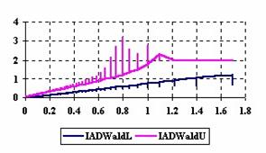
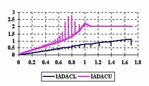
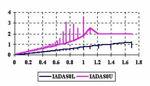
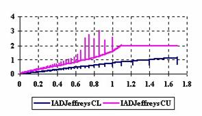
Figure 1. The upper and lower confidence limits (logarithmic scale) for
number needed to treat/harm at 0 < X, Y < m = n = 50
The SlideWrite Plus graphical representations (figure 2) were create using a 3D-Mesh graph type with 80% perspective, 25° tilt angle, and 60° rotation angle. On X-axis were represented the X values, on the Y-axis the Y values and on the Z-axis the number needed to treat/harm, the lower or the upper confidence intervals or the experimental errors, according to the experiment. There were represented with red color the experimental values from 0 to 2, with green the values from 2 to 4, with blue the values from 4 to 6, with cyan the values from 6 to 8, and with magenta the values from 8 to 10.
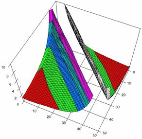
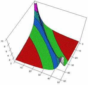
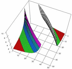

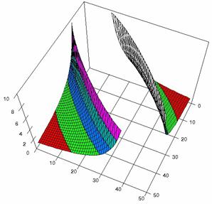
Figure 2. The number needed to treat/harm and its confidence intervals limits
with IADWald and IADJeffreysC at n = m = 50
The averages and standard deviations of the experimental errors for number needed to treat/harm for different equal samples sizes (m = n = 10, 20, and 30) were report in table 1.
|
n |
IADWald |
IADAC |
IADAS0 |
IADJeffreysC |
|
10 |
5.16 (3.89) |
1.69 (0.90) |
2.97 (1.71) |
2.02 (1.11) |
|
20 |
4.39 (2.77) |
2.40 (1.20) |
3.55 (1.53) |
3.19 (1.69) |
|
30 |
4.24 (2.27) |
2.71 (1.25) |
3.54 (1.52) |
3.57 (1.80) |
Table 1. The averages of experimental errors and standard deviations (parentheses) for NNT/NNH at m = n = 10, 20, and 30
The graphical representations of the experimental errors for m = n = 10 were presented in figure 3, for m = n = 20 in figure 4, for m = n = 30 in figure 5.
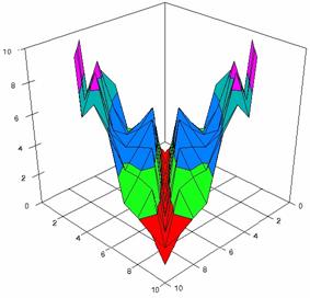
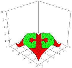
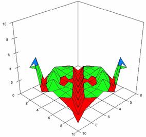
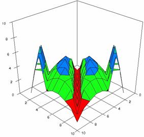
Figure 3. The percentages of experimental errors obtained NNT/NNH with IADWald, IADAC, IADAS0 and IADJeffreysC at 0 < X, Y < m = n = 10
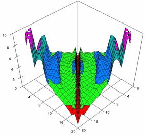
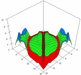
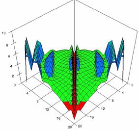
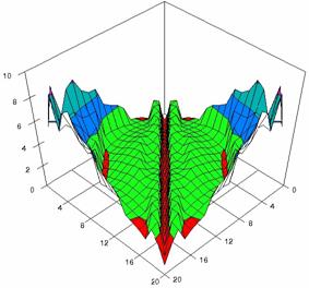
Figure 4. The percentages of experimental errors for NNT/NNH with IADWald, IADAC, IADAS0, and IADJeffreysC at 0 < X, Y < m = n = 20
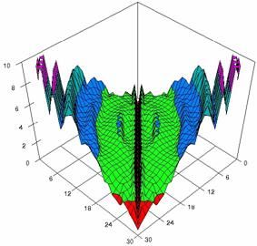
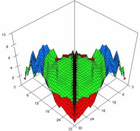
Figure 5. The percentages of experimental errors NNT/NNH with IADWald, and IADAC
at 0 < X, Y < m = n = 30
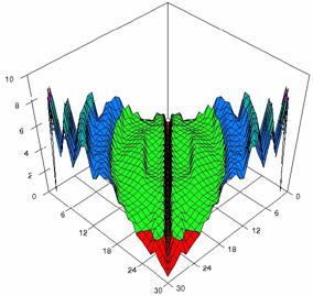
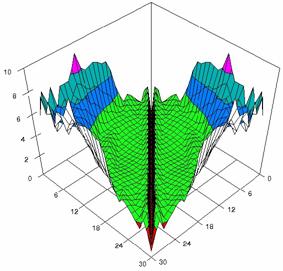
Figure 5. The percentages of experimental errors for NNT/NNH with IADAS0, and IADJeffreysC at 0 < X, Y < m = n = 30
The assessment of the confidence intervals methods was carries on with a particular situation: X = 3·m/4 and Y = 1·n/4 at equal (m = n = 4, 8, 12..204) sample sizes. The experimental results were import in Microsoft Excel where the graphical representations were creates (figure 6). In the graphical representation, on horizontal axis were represent the m = n values depending on X and Y values and on the vertical axis the percentage of the experimental errors.
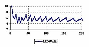
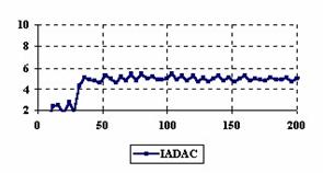
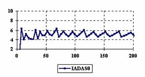
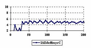
Figure 6. The variation of the experimental errors for number needed to treat/harm
at X = 3·m/4, Y = 1·n/4, 2 < X < 154, and 0 < Y < 52 at m = n = 4,8..204
The averages (MErr) and standard deviations (StdDev) of experimental errors for X = 3·m/4 and Y = 1·n/4 at equal (m = n = 4, 8, 12..204) sample sizes were presented in table 3.
|
Method |
IADWald |
IADAC |
IADAS0 |
IADJeffreysC |
|
MErr |
5.57 |
4.55 |
5.04 |
4.47 |
|
StdDev |
0.91 |
1.20 |
0.90 |
1.12 |
Table 2. The averages and standard deviations of experimental error for
X = 1/4/m and Y = 3/4/n and 2< X<154 and 0<Y<52 when m = n = 4,8..204
The surface plots of dependences of the average of deviations relative to significance level α = 5% (Var5) at m = 4..14 and n = 4..14 were graphically represent in figure 7.
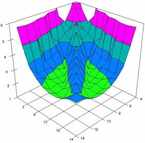
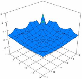
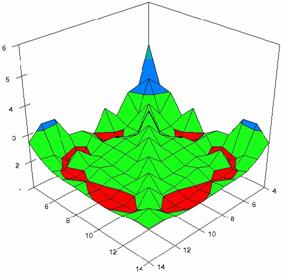
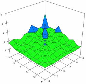
Figure 7. Dependences of the deviations relative to the significance level α = 5% for NNT/NNH with IADWald, IADAC, IADAS0, IADJeffreysC at m, n = 4..14
In the figure 7 were represent with red color the experimental values from 1 to 2, with green from 2 to 3, with blue from 3 to 4, with cyan from 4 to 5, and with magenta from 5 to 6.
The averages of the deviations relative to the imposed significance level α = 5% (MDev5) for sample sizes (m, n) which vary in 4..14 domain were: for IADWald MDev5 = 4.43, for IADAC MDev5 = 3.41, for IADAS0 MDev5 = 2.30, and for IADJeffreysC MDev5 = 2.67.
Using the results from the random variable (X, Y) and random samples sizes (n, m) when 1 ≤ X, Y < n, m and 4 ≤ n, m ≤ 1000 a set of calculation were perform and graphical represent in figure 8.
Figure 8 contains the frequencies of the experimental error (black dots) for each specified method, the best errors interpolation curve with a Gauss curve (dIG(er), green line), the Gauss curves of the average and standard deviation of the experimental errors (dMV(er), red line), the Gauss curve of the experimental errors deviations relative to the significance level (d5V(er), blue squares), and the Gauss curve of the standard binomial distribution relative to an average of the experimental errors equal with 100·α (pN(er,10), black line).
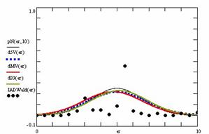
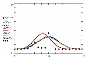
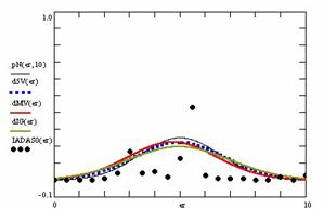
Figure 8. The pN(er, 10), d5V(er), dMV(er), dIG(er) and the frequencies of the experimental errors for random variables and sample sizes (1 ≤ X,Y < 1000, 4 ≤ m, n ≤ 1000)
For the random samples (m, n) and random binomial variables (X, Y), the results were present in tables 3 - 6. Table 3 contains the averages of the deviation of the experimental errors relative to significance level α =5% (Dev5), the absolute differences of the average of experimental errors relative to the imposed significance level (|5-M|), and standard deviations (StdDev).
|
No |
Method |
Dev5 |
Method |
|5-M| |
Method |
StdDev |
|
1 |
IADAC |
1.46 |
IADWald |
0.24 |
IADAC |
1.20 |
|
2 |
IADAS0 |
1.79 |
IADAS0 |
0.29 |
IADAS0 |
1.77 |
|
3 |
IADWald |
1.84 |
IADAC |
0.84 |
IADWald |
1.82 |
Table 3. Methods ordered by performance according to Dev5, |5-M| and StdDev criterions
Table 4 contains the absolute differences of the averages that result from Gaussian interpolation curve to the imposed significance level (|5-MInt|), the deviations that result from Gaussian interpolation curve (DevInt), the correlation coefficient of interpolation (r2Int) and the Fisher point estimator (FInt).
|
No |
Method |
|5-MInt| |
Method |
DevInt |
Method |
r2Int |
FInt |
|
1 |
IADAS0 |
0.03 |
IADAC |
1.57 |
IADAS0 |
0.41 |
13 |
|
2 |
IADAC |
0.11 |
IADWald |
1.74 |
IADWald |
0.45 |
15 |
|
3 |
IADWald |
0.15 |
IADAS0 |
2.02 |
IADAC |
0.53 |
22 |
Table 4. The methods ordered by |5-Mint|, DevInt, r2Int and FInt criterions
The superposition between the standard binomial distribution curve and interpolation curve (pNIG), the standard binomial distribution curve and the experimental error distribution curve (pNMV), and the standard binomial distribution curve and the error distribution curve around significance level (pN5V) were present in table 5.
|
No |
Method |
pNIG |
Method |
pNMV |
Method |
pN5V |
|
1 |
IADAS0 |
0.88 |
IADAC |
0.74 |
IADWald |
0.93 |
|
2 |
IADWald |
0.94 |
IADWald |
0.91 |
IADAS0 |
0.94 |
|
3 |
IADAC |
0.97 |
IADAS0 |
0.92 |
IADAC |
0.96 |
Table 5. The confidence intervals methods ordered by the
pIGMV, pIG5V, and pMV5V criterions
Table 6 contains the percentages of superposition between interpolation Gauss curve and the Gauss curve of error around experimental mean (pIGMV), between the interpolation Gauss curve and the Gauss curve of error around imposed mean (α = 5%) (pIG5V), and between the Gauss curve experimental error around experimental mean and the error Gauss curve around imposed mean α = 5% (pMV5V).
|
No |
Method |
pIGMV |
Method |
pIG5V |
Method |
pMV5V |
|
1 |
IADAS0 |
0.92 |
IADAC |
0.96 |
IADWald |
0.94 |
|
2 |
IADWald |
0.91 |
IADWald |
0.96 |
IADAS0 |
0.93 |
|
3 |
IADAC |
0.77 |
IADAS0 |
0.94 |
IADAC |
0.74 |
Table 6. The confidence intervals methods ordered by the
pIGMV, pIG5V, and pMV5V criterions
Discussions
Analyzing the results of the experiments for equal sample sizes, it can be observe that the best estimation, if we look after a method which to obtained an average of the experimental errors closed 100· α, is the IADWald method for m = n = 10. Contrary with this performance, the IADWald obtained the greatest standard deviation of experimental errors compared with the IADAC, IADAs0 and IADJeffreysC methods. The lowest standard deviation for m = n = 10 is obtains by the IADAC method. For the IADAC, IADAs0 and IADJeffreysC methods the average of the experimental errors were increase with n but these averages did not exceed the imposed significance level (α = 5%). Contrary, the experimental errors average obtained with IADWald method were decrease with increasing of sample size. The lowest experimental standard deviation was obtains systematically by the IADAC method.
Looking at the results for X = 3·m/4 and Y = 1·n/4 and m = n = 4, 8, 12,..204 the IADAs0 method obtained an average of the experimental errors closest to the imposed significance level α = 5% (5.04%), and the lowest standard deviation (0.90).
When the sample sizes varies from 4 to 14 (4 ≤ m, n < 14), the IADAS0 method obtain the lowest deviation relative to the impose significance level (α = 5%). The IADWald method have the highest deviation of the experimental errors in confidence intervals estimation for NNT/NNH when 4 ≤ m, n < 14.
Analyzing the results obtained from the random samples (m, n random numbers from the range 4..1000) and random binomial variables (X, Y) it can be remark that the IADWald method obtained the lowest absolute differences of the average of experimental errors relative to the imposed significance level (100·α). The lowest experimental standard deviation and experimental deviation to the significance level (α = 5%) was obtains by the IADAC method.
The IADAs0 method obtained the closest interpolation average to the significance level (table 5). The lowest interpolation standard deviation and the best correlation between theoretical curve and experimental data was obtains by the IADAC method.
The IADAC method obtained the maximum superposition between the curve of interpolation and the curve of standard binomial distribution and the maximum superposition between the curve of standard binomial distribution and the curve of errors around the significance level (α = 5%). The maximum superposition between the curve of standard binomial distribution and the curve of experimental error distribution was obtains by the IADAS0 method.
The maximum superposition between the Gauss curve of interpolation and the Gauss curve of errors around experimental mean was obtains by the IADAS0 method. The IADAC method obtained again the maximum superposition between the Gauss curve of interpolation and the Gauss curve of error around significance level (α = 5%). The IADWald method obtained the maximum superposition between Gauss curve of experimental errors and the Gauss curve of errors around imposed mean (α = 5%).
Conclusions
All implemented methods of computing confidence intervals for number needed to treat/harm obtain performances and present different behaviors in different situation. For equal sample sizes (m = n) most of the implemented methods present an increase of the experimental errors averages with increasing of the equals sample sizes except the IADWald which present a decrease of the experimental errors with increasing of the sample sizes.
The average and the deviation relative to the imposed significance level of the experimental errors on random variables (X, Y) and random sample sizes (m, n) could be consider the best criterions of assessment. Thus, we can say the IADAC method obtained systematically performance in confidence intervals estimation for number needed to treat/harm, even if we look after the experimental errors, the standard deviation, or the deviation relative to the significance level, closely followed by the IADAS0 method.
We recommend the IADAC and IADAS0 methods to be taking into consideration when confidence intervals for number needed to treat /harm is necessary.
Acknowledgements
The first author is thankful for useful suggestions and all software implementation to Ph. D. Sci., M. Sc. Eng. Lorentz JÄNTSCHI from Technical University of Cluj-Napoca.
References