Pearson versus Spearman, Kendall's Tau Correlation Analysis on Structure-Activity Relationships of Biologic Active Compounds

Sorana-Daniela BOLBOACĂ¹, Lorentz JÄNTSCHI ²

¹“Iuliu Haţieganu” University of Medicine and Pharmacy, 13 Emil Isac, 400023 Cluj-Napoca, Romania;  ²Technical University of Cluj-Napoca, 15 Constantin Daicoviciu, 400020 Cluj-Napoca, Romania

sbolboaca@umfcluj.ro, lori@academicdirect.org,

Abstract

A sample of sixty-seven pyrimidine derivatives with inhibitory activity on E. coli dihydrofolate reductase (DHFR) was studied by the use of molecular descriptors family on structure-activity relationships. Starting from the results obtained by applying of MDF-SAR methodology on pyrimidine derivatives and from the assumption that the measured activity (compounds’ inhibitory activity) of a biologically active compounds is a semi-quantitative outcome (can be related with the type of equipment used, the researchers, the chemical used, etc.), the abilities of Pearson, Spearman, Kendall’s, and Gamma correlation coefficients in analysis of estimated toxicity were studied and are presented.

Keywords

Multiple linear regressions, Correlation coefficients, Molecular Descriptors Family on Structure-Activity Relationships (MDF-SAR)

Introduction

QSAR (Quantitative Structure-Activity Relationships) is an approach which is able to indicate for a given compound or a class of compounds which feature of structure characteristics is correlated with its activity [1]. In QSAR analysis were proposed several approaches for development. Simple and multiple linear regressions is one of the more successful techniques use by many researcher in construct of QSAR models [2]-,[3],[4].

Correlation coefficient is a simple statistical measure of relationship between one dependent and one or more than one independent variables and it is use as a measure of the statistical fit of a regression based model in QSAR [5]. Its squared value (the coefficient of determination) it is most frequently used parameter as a measure of the goodness-of-fit of the model [6]-,[7],[8],[9],[10].

A new approach of molecular descriptors family on structure-activity relationships (MDF-SAR) was developed [11], and proved its usefulness in estimation and prediction of: toxycity [12], [13], mutagenicity 12, antioxidant efficacy [14], antituberculotic activity [15], antimalarial activity [16], antiallergic activity [17], anti-HIV-1 potencies [18], inhibition activity on carbonic anhydrase II [19] and IV [20].

Several correlation coefficients based on different statistical hypothesis are known and most frequently used today: Pearson correlation coefficient, Spearman rank correlation coefficient and Spearman semi-quantitative correlation coefficient, Kendall tau-a, -b and -c correlation coefficients, Gamma correlation coefficient 5.

Starting from the results obtained by applying of MDF-SAR methodology on a sample of sixty-seven compounds and from the assumption that the measured activity (compounds’ inhibitory activity) of a biologically active compounds is a semi-quantitative outcome (can be related with the type of equipment used, the researchers, the chemical used), the abilities of Pearson, Spearman, Kendall’s, and Gamma correlation coefficients in analysis of estimated toxicity were studied.

Multi-varied MDF-SAR model of pyrimidine derivatives

A sample of sixty-seven pyrimidine derivatives with inhibitory activity on E. coli dihydrofolate reductase (DHFR) was studied by the use of MDF-SAR methodology.

The set of pyrimidine derivatives (2,4-Diamino-5-(substituted-benzyl)-pyrimidine derivatives) with inhibitory activity on E. coli dihydrofolate reductase (DHFR) was  previously studied by Ting-Lan Chiu & Sung-Sau So by the use of neural network approach [21].

By applying the MDF-SAR methodology on the sample of sixty-seven pyrimidine derivatives, a multi-varied model with four descriptors reveled to has good performances in prediction and estimation of inhibitory activity.

The multi-varied MDF-SAR model with four descriptors had the following equation:

Y_est = 3.78 + 1.62·iImrKHt + 2.37·liMDWHg + 6.40·IsDrJQt - 8.52·10^-2·LSPmEQg

Analyzing the MDF-SAR model with four descriptors it could be say that inhibitory activity consider compounds geometry (g) and topology (t), being related with the number of directly bonded hydrogen’s (H) of compounds and with the partial charge (Q) as atomic properties.

Statistical characteristics of the MDF-SAR model with four descriptors are in table 1 and 2.

Table 1. Statistical characteristics of the multi-varied MDF-SAR model with four descriptors

Characteristic (notation)	Value
Number of variable (v)	4
Correlation coefficient (r)	0.9517
95% Confidence Intervals for r (95% CIr)	[0.9223, 0.9701]
Squared correlation coefficient (r^2)	0.9058
Adjusted squared correlation coefficient (r^2adj)	0.8997
Standard error of estimated (sest)	0.1919
Fisher parameter (Fest)	149^*
Cross-validation leave-one-out (loo) score (r^2cv-loo)	0.8932
Fisher parameter for loo analysis (Fpred)	130^*
Standard error for leave-one-out analysis (sloo)	0.2044
Model stability (r^2 - r^2cv(loo))	0.0126
r^2(iImrKHt, liMDWHg)	0.2020
r^2(iImrKHt, IsDrJQt)	0.0047
r^2(iImrKHt, LSPmEQg)	0.1482
r^2(liMDWHg, IsDrJQt)	0.0003
r^2(liMDWHg, LSPmEQg)	0.0212
r^2(IsDrJQt, LSPmEQg)	0.0664
^*p < 0.001

Table 2. Statistics of the regression MDF-SAR model with four descriptors

	StdError	t Stat	95%CIcoefficient	r(Ym,desc)
Intercept	0.1999	18.92^*	[3.38, 4.18]	n.a.
iImrKHt	0.0709	22.85^*	[1.48, 1.76]	0.4803
liMDWHg	0.1500	15.81^*	[2.07, 2.67]	0.0558
IsDrJQt	1.4779	4.33^*	[3.45, 9.36]	0.0336
LSPmEQg	0.0182	-4.68^*	[-0.12, -0.12]	0.0231
StdError = standard error; t Stat = Student tets parameter; 95% CIcoefficient = 95% confidence interval associated with regression coefficients; Ym = measured inhibitory activity; desc = molecular descriptor; ^* p < 0.001

Graphical representation of the measured versus estimated by MDF-SAR model with four descriptors inhibitory activity is in figure 1.

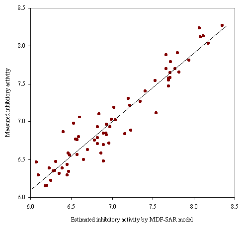
Figure 1. Plot of measured vs estimated by MDF-SAR inhibitory activity

Internal validation of the four-varied MDF SAR model with four descriptors was performed through splitting the whole set into training and test sets by applying of a randomization algorithm.

The coefficients for each model obtained in training sets, in conformity with the generic equation Y_est = a₀ + a₁·iImrKHt + a₂·liMDWHg + a₃·IsDrJQt - a₄·10^-2·LSPmEQg, the number of compounds in training (N_tr) and test (N_ts) sets, the correlation coefficient for training (r_tr) and test (r_ts) sets with associated 95% confidence intervals (95%CI_rtr and 95%CI_rts), the Fisher parameter associated with training (F_tr) and test (F_ts) sets, and the Fisher’s Z parameter of correlation coefficients comparison (Zrtr-rts) are in table 3.

Table 3. Statistics results on training versus test sets

a0	a1	a2	a3	a4	Ntr	rtr	95%CIrtr	Ftr	Nts	rts	95%CIts	Fts	Zrtr-rts
3.93	1.61	2.43	6.56	-9.67·10^-2	35	0.949	[0.899, 0.974]	67^*	32	0.958	[0.916, 0.980]	59^*	0.418^†
3.98	1.57	2.45	6.55	-7.52·10^-2	36	0.951	[0.905, 0.975]	73^*	31	0.951	[0.899, 0.976]	61^*	0.000^†
3.84	1.55	2.15	9.08	-9.12·10^-2	37	0.944	[0.893, 0.908]	66^*	30	0.949	[0.895, 0.976]	55^*	0.206^†
3.94	1.59	2.42	6.10	-8.18·10^-2	38	0.951	[0.907, 0.974]	78^*	29	0.947	[0.890, 0.975]	50^*	0.144^†
3.91	1.56	2.25	8.22	-1.04·10^-1	39	0.963	[0.931, 0.981]	110^*	28	0.937	[0.867, 0.971]	39^*	1.069^†
4.18	1.51	2.44	6.06	-7.22·10^-2	40	0.956	[0.917, 0.975]	92^*	27	0.936	[0.863, 0.971]	35^*	0.721^†
3.76	1.63	2.32	7.35	-1.02·10^-1	41	0.963	[0.931, 0.980]	116^*	26	0.935	[0.858, 0.971]	34^*	1.104^†
3.97	1.58	2.39	5.11	-9.36·10^-2	42	0.956	[0.919, 0.976]	99^*	25	0.954	[0.896, 0.980]	34^*	0.115^†
3.64	1.64	2.30	7.00	-8.15·10^-2	43	0.955	[0.917, 0.975]	98^*	24	0.944	[0.873, 0.976]	37^*	0.407^†
3.72	1.66	2.43	5.78	-8.12·10^-2	44	0.938	[0.889, 0.966]	72^*	23	0.964	[0.916, 0.985]	54^*	1.030^†
3.59	1.64	2.25	4.94	-9.98·10^-2	45	0.947	[0.904, 0.970]	86^*	22	0.957	[0.898, 0.982]	37^*	0.411^†
3.86	1.55	2.23	8.68	-8.86·10^-2	46	0.940	[0.894 0.967]	78^*	21	0.983	[0.958, 0.993]	43^*	2.290^*
4.04	1.54	2.36	6.46	-7.31·10^-2	47	0.949	[0.911, 0.972]	96^*	20	0.963	[0.906, 0.985]	34^*	0.538^†
3.63	1.63	2.24	4.27	-8.93·10^-2	48	0.940	[0.895, 0.966]	82^*	19	0.963	[0.904, 0.986]	44^*	0.852^†
3.98	1.57	2.42	6.49	-8.59·10^-2	49	0.946	[0.905, 0.969]	93^*	18	0.960	[0.894, 0.985]	36^*	0.535^†
3.77	1.61	2.32	6.37	-8.46·10^-2	50	0.943	[0.902, 0.968]	91^*	17	0.974	[0.927, 0.991]	52^*	1.294^†
3.67	1.63	2.22	6.56	-1.01·10^-1	51	0.954	[0.919, 0.973]	115^*	16	0.950	[0.858, 0.983]	17^*	0.126^†
3.81	1.61	2.39	6.87	-7.70·10^-2	52	0.951	[0.916, 0.972]	112^*	15	0.950	[0.853, 0.984]	22^*	0.032^†
3.69	1.65	2.36	6.32	-8.21·10^-2	53	0.953	[0.919, 0.972]	118^*	14	0.956	[0.864, 0.986]	17^*	0.128^†
3.97	1.56	2.40	6.16	-7.51·10^-2	54	0.951	[0.916, 0.971]	115^*	13	0.954	[0.851, 0.987]	17^*	0.122^†
^† p > 0.05; ^* p < 0.01

Definitions, Formulas, Interpretations, PHP functions, and Results

A number of add notations were used in the study, as follows:

· Pearson product-moment correlation coefficient (named after Karl Pearson (1857 - 1936), a major contributor to the early development of statistics):

o r_prs = the Pearson correlation coefficient;

o r_Prs² = the squared Pearson correlation coefficient;

o t_Prs,df = the Student test parameter, and its significance p_Prs,df at a significance level of 5% (where df = the degree of freedom);

· Spearman’s rank correlation coefficient (named after Charles Spearman (1863 - 1945), English psychologist known for his work in statistics - factor analysis, and Spearman's rank correlation coefficient):

o r_Spm = the Spearman rank correlation coefficient

o r_Spm² = the squared of Spearman rank correlation coefficient;

o t_Prs,df = the Student test parameter, and its significance p_Spm,df;

o r_sQ² = the squared of Spearman semi-Qantitative correlation coefficient;

o t_sQ = the Student test parameter, and its significance p_sQ;

· Kendall’s tau correlation coefficients (named after Maurice George Kendall (1907 - 1983), a prominent British statistician; published in monograph Rank Correlation in 1948);

o τ_Ken,a = the Kendall tau-a correlation coefficient;

o τ_Ken,a² = the squared of Kendall tau-a correlation coefficient;

o Z_Ken,τa = the Z-test parameter of Kendall tau-a correlation coefficient, and its significance p_Ken,τa;

o τ_Ken,b = the Kendall tau-b correlation coefficient;

o τ_Ken,b² = the squared of Kendall tau-b correlation coefficient;

o Z_Ken,τb = the Z-test parameter of Kendall tau-b, and its significance p_Ken,τb;

o τ_Ken,c² = the Kendall tau-c correlation coefficient;

o τ_Ken,c² = the squared of Kendall tau-c correlation coefficient;

o Z_Ken,τc = the Z-test parameter of Kendall tau-c, and its significance p_Ken,τc;

· Gamma correlation coefficient (also known as Goodman and Kruskal's gamma):

o Γ = the Gamma correlation coefficient;

o Γ² = the squared of Gamma correlation coefficient;

o Z_Γ = the Z-test parameter of Gamma correlation coefficient, and its significance p_Γ.

A series of *.php programs which to facilitate the calculation and to display of above-described correlation coefficients and their statistics (Student-test and Z-test parameters and associated significances) were implemented and was use in order to reach the objective of study [22].

Pearson correlation coefficient

Definition: a measure the strength and direction of the linear relationship between two variables, describing the direction and degree to which one variable is linearly related to another.

Assumptions: both variable (variables Y_m and Y_est) are interval or ratio variables and are well approximated by a normal distribution, and their joint distribution is bivariate normal [23].

Formula

where Y_m-i is the value of the measured inhibitory activity for compound i (i = 1, 2, …, 67)  is the average of the measured inhibitory activity, Y_est-i is the value of the estimated inhibitory activity for compound i, and  is the average of the estimated inhibitory activity.

Interpretation

The Pearson correlation coefficient can take values from -1 to +1. A value of +1 show that the variables are perfectly linear related by an increasing relationship, a value of -1 show that the variables are perfectly linear related by an decreasing relationship, and a value of  0 show that the variables are not linear related by each other. There is considered a strong correlation if the correlation coefficient is greater than 0.8 and a weak correlation if the correlation coefficient is less than 0.5.

The coefficient of determination (or r squared) gives information about the proportion of variation in the dependent variable which might be considered as being associated with the variation in the independent variable.

Related statistics:

· The squared of Pearson correlation coefficient or Pearson coefficient of determination (r_Prs²);

o Describe the proportion of variance in Y_m that is related with linear variation of Y_est;

o Can take values from 0 to 1.     

Statistical test

Student t-test was used to determine if the value of Pearson correlation coefficient is statistically significant, at a significance level of 5%.

The null hypothesis vs. the alternative hypothesis was:

H₀: r_Prs = 0 (there is no correlation between the variables)

H₁: r_Prs < > 0 (variables are correlated)

For a significance level equal with 5%, a p-value associated to t_Prs,df less than 0.05 means that there is evidence to reject the null hypothesis in favor of the alternative hypothesis. In other words there is a statistically significant linear relationship between the variables.

PHP implementation

In order to compute the statistics associated with Pearson correlation coefficient, three functions were implemented:

function coef_rk(&$y1,&$y2){

  $my1=m1($y1);

  $dy2=m2($y1,$y1)-$my1*$my1;

  $mx1=m1($y2);

  $mxy=m2($y2,$y1);

  $m2x=$mx1*$mx1;

  $mx2=m2($y2,$y2);

  $dx2=$mx2-$m2x;

  $r2=pow($mxy-$mx1*$my1,2)/($dx2*$dy2);

  return $r2;

}

function t_p($n,$k,$r){

  return $r*pow($n-$k-1,0.5)/pow(1-pow($r,2),0.5);

}

function p_t($t,$df){

  $p = $df/2;

  $x = 0.5+0.5*$t/pow(pow($t,2)+$df,0.5);

  $beta_gam = exp( -logBeta($p, $p) + $p * log($x) + $p * log(1.0 - $x) );

  return (2.0 * $beta_gam * betaFraction(1.0 - $x, $p, $p) / $p);

}

The statistics of Pearson correlation coefficients are computed as follows:

· Pearson correlation coefficient:

$r_pe = coef_rk($cmp[0],$cmp[1]);

where $cmp[0] is the measured inhibitory activity (Y_m), and $cmp[1] is the estimated by MDF-SAR model with four descriptor inhibitory activity (Y_est).

· t Student parameter:

$t_pe = t_p($n,1,pow($r_pe,0.5));

· Significance of t Student parameter

$p_pe = p_t($t_pe,$n-2);

Results:

r_Prs² = 0.9058

t_Prs,1 = 24.99                                                                                                     (1)

p_Prs,1 = 4.74·10^-33 %

Spearman’s rank correlation coefficient

Definition: a non-parametric measure of correlation between variable which assess how well an arbitrary monotonic function could describe the relationship between two variables, without making any assumptions about the frequency distribution of the variables. Frequently the Greek letter ρ (rho) is use to abbreviate the Spearman correlation coefficient.

Spearman’s rank correlation is satisfactory for testing the null hypothesis of no relationship, but is difficult to interpret as a measure of the strength of the relationship [24].

Assumptions:

· Does not required any assumptions about the frequency distribution of the variables;

· Does not required the assumption that the relationship between variable is linear;

· Does not required the variable to be measured on interval or ration scale.

Formula

In order to compute the Spearman rank correlation coefficient, the two variables (Y_m, respectively Y_est) were converted to ranks (see table 4 for exemplification). For each measured and estimated inhibitory activity a rank was assigned (RankY_m - for measure inhibitory activity, RankY_est - for estimated by MDF-SAR model inhibitory activity) according with the position of value into a sort serried of values.

In assignment of rank process, the lowest value had the lowest rank. When there are two equal values for two different compounds (for measured and/or estimated inhibitory activity), the associated rank had equal values and was calculated as means of corresponding ranks. For example, the compounds abbreviated as c_52 and c_59 have the same measured inhibitory activity (6.45, see table 4). The rank associated with these values is equal with 13.5 (is the average between the rank for c_52 - 13 and the rank of c_59 - 14).

Table 4. Compounds abbreviation, measured and estimated activity and associated ranks

Abb.	Ym	RankYm		Yest	RankYest	Abb.	Ym	RankYm		Yest	RankYest
c_64	6.07	1	0	6.4626	13	c_32	6.92	35	0	6.8423	32
c_65	6.10	2	0	6.2948	5	c_66	6.93	36.5	5	6.8225	30
c_67	6.18	3	0	6.1479	1	c_36	6.93	36.5		6.9609	38
c_54	6.20	4	0	6.1595	2	c_40	6.96	38	0	6.7150	24
c_37	6.23	5	0	6.3859	10	c_17	6.97	39	0	6.9298	36
c_48	6.25	6	0	6.2254	3	c_45	6.99	40	0	7.0283	41
c_31	6.28	7	0	6.3483	8	c_41	7.02	41	0	7.1919	45
c_49	6.30	8	0	6.3528	9	c_15	7.04	42	0	7.0225	40
c_10	6.31	9	0	6.4703	14	c_28	7.16	43	0	6.8355	31
c_56	6.35	10	0	6.3149	6	c_09	7.20	44	0	7.3115	48
c_47	6.39	11	0	6.3866	11	c_18	7.22	45	0	7.2156	46
c_53	6.40	12	0	6.8614	34	c_43	7.23	46	0	6.8855	35
c_52	6.45	13.5	1	6.2913	4	c_29	7.35	47	0	7.2724	47
c_59	6.45	13.5		6.4336	12	c_14	7.41	48	0	7.4072	49
c_16	6.46	15	0	6.5851	20	c_24	7.53	49	0	7.5476	51
c_34	6.47	16	0	6.3422	7	c_22	7.54	50	0	7.1218	44
c_58	6.48	17	0	6.5536	17	c_26	7.66	51.5	6	7.7002	57
c_35	6.53	18	0	6.9755	39	c_08	7.66	51.5		7.8841	61
c_42	6.55	19	0	6.7654	27	c_27	7.69	54	7	7.4715	50
c_30	6.57	20.5	2	6.5625	18	c_13	7.69	54		7.5489	52
c_61	6.57	20.5		6.7594	26	c_12	7.69	54		7.5793	53
c_33	6.59	22	0	6.8010	29	c_04	7.71	56.5	8	7.5841	54
c_51	6.60	23	0	7.0616	42	c_11	7.71	56.5		7.6497	55
c_39	6.65	24	0	6.4993	16	c_19	7.72	58	0	7.7915	59
c_38	6.70	25	0	6.6297	21	c_23	7.77	59	0	7.7014	58
c_57	6.78	26	0	6.7552	25	c_25	7.80	60	0	7.9130	62
c_60	6.82	28	3	6.7091	23	c_01	7.82	61	0	7.6576	56
c_44	6.82	28		6.7847	28	c_21	7.94	62	0	7.8130	60
c_55	6.82	28		6.9318	37	c_06	8.07	63	0	8.2391	66
c_20	6.84	30	0	7.1067	43	c_03	8.08	64	0	8.1224	64
c_46	6.86	31	0	6.5813	19	c_07	8.12	65	0	8.1353	65
c_50	6.89	33	4	6.4794	15	c_05	8.18	66	0	8.0372	63
c_62	6.89	33		6.6942	22	c_02	8.35	67	0	8.2702	67
c_63	6.89	33		6.8475	33

The method of rank assignment for more then two equal values of measured and/or estimated inhibitory activity is the same as for two equal values. If there are an odd number of compounds which have the same measured value (see compounds c_60, c_44, and c_55 from table 2) then the rank will be an integer ((27+28+29)/3 = 28, see the rank for c_60, c_44, and c_55).

In studied example, there are equal values for measured activity: five situations of two equal values (c_52-c_59, c_30-c_61, c_66-c_36, c_26-c_08, and c_04-c_11), and three situations of three equal values (c_60-c_44-c_55, c_50-c_62-c_63, and c_27-c_13-c_12).

By conversion of the measured and estimated inhibitory activity to ranks, the distribution of ranks does not depend on the distribution of measured, respectively estimated inhibitory activity.

The formula for calculation of the Spearman rank correlation coefficient is:

where R_Ym-i is the rank of the measured inhibitory activity for compound i,  is the average of the measured inhibitory activity, R_Yest-i is the rank of the estimated by MDF-SAR inhibitory activity for compound i, and  is the average of the estimated inhibitory activity.

The simple formula for r_Spm is based on the difference between each pairs of ranks:

where D is the differences between each pair of ranks (e.g. D = R_Ym-1 - R_Yest-1) and n is the volume of the sample.

The formula of the Spearman semi-quantitative method is:

Interpretation

· Identical with Pearson correlation coefficient.

Related statistics:

· r_Spm² = the squared of Spearman rank correlation coefficient;

· r_sQ² = the squared of semi-quantitative correlation coefficient.

Statistical significance:

· Compute by the use of a permutation test (a statistical test in which the reference distribution is obtained by permuting the observed data points across all possible outcomes, given a set of conditions consistent with the null hypothesis);

· Comparing the observed r_Spm with published tables for different levels of significance (eg. 0.05, 0.01…). It is a simple solution when the researchers want to know the significance within a certain range or less than a certain value;

· Tested by applying the Student t-test (for sample sizes > 20): the method used in this study.

The null hypothesis vs. the alternative hypothesis for Spearman rank correlation coefficient was:

H₀: r_Spm = 0 (there is no correlation between the ranked pairs)

H₁: r_Spm < > 0 (ranked pairs are correlated)

The null hypothesis vs. the alternative hypothesis for semi-quantitative correlation coefficient was:

H₀: r_sQ = 0 (there is no correlation between the ranked pairs)

H₁: r_sQ < > 0 (ranked pairs are correlated)

PHP implementation

The formulas for Spearman and respectively semi-quantitative correlation coefficients used two defined above functions (t_p and respectively p_t). The Spearman rank correlation coefficient used the coef_rk function defined as:

function coef_rk(&$y1,&$y2){

  $my1=m1($y1);

  $dy2=m2($y1,$y1)-$my1*$my1;

  $mx1=m1($y2);

  $mxy=m2($y2,$y1);

  $m2x=$mx1*$mx1;

  $mx2=m2($y2,$y2);

  $dx2=$mx2-$m2x; 

  $r2=pow($mxy-$mx1*$my1,2)/($dx2*$dy2);

  return $r2;

}

where

function m1(&$v){

 $rez=0;

 $n=count($v);

 for($i=1;$i<$n;$i++)

  $rez+=$v[$i];

 return $rez/($n-1);

}

function m2(&$v,&$u){

 $rez=0;

 $n=count($v);

 for($i=1;$i<$n;$i++)

  $rez+=$v[$i]*$u[$i];

 return $rez/($n-1);

}

Spearman correlation coefficient

The statistics of Spearman rank correlation coefficients are computed as follows:

· Spearman correlation coefficient:

$r_sp = coef_rk($poz[0],$poz[1]);

where $poz[0] is the position on sort series of measured inhibitory activity, and $poz[1] is the position on sort serried of estimated inhibitory activity by MDF-SAR model with four descriptor.

· t Student parameter:

$t_sp = t_p($n,1,pow($r_sp,0.5));

· Significance of t Student parameter

$p_sp = p_t($t_sp,$n-2);

Semi-quantitative correlation coefficient

The statistics of semi-quantitative correlation coefficients are computed as follows:

· Semi-quantitative correlation coefficient:

$r_sq = pow($r_pe*$r_sp,0.5);

· t Student parameter:

$t_sq = t_p($n,1,pow($r_sq,0.5));

· Significance of t Student parameter

$p_sq = p_t($t_sq,$n-2);

Results:

r_Spr² = 0.8606

t_Spm,1 = 20.03                                                                                                   (2)

p_Spm,1 = 1.62·10^-29

r_sQ² = 0.8829

t_sQ = 22.14                                                                                                       (3)

p_sQ = 5.57·10^-32

Kendall’s rank correlation coefficients

Definition

Kendall-tau is a non-parametric correlation coefficient that can be used to assess and test correlations between non-interval scaled ordinal variables. Frequently the Greek letter τ (tau), is use to abbreviate the Kendall tau correlation coefficient.

The Kendall tau correlation coefficient is considered to be equivalent to the Spearman rank correlation coefficient. While Spearman rank correlation coefficient is like the Pearson correlation coefficient but computed from ranks, the Kendall tau correlation rather represents a probability.

There are three Kendall’s tau correlation coefficient known as tau-a, tau-b, and tau-c.

Formula

Let (Y_m-i, Y_est-i) and (Y_m-j, Y_est-j) be the pair of measured and estimated inhibitory activity. If Y_m-j - Y_m-i and Y_est-j - Y_est-i, where i < j have the same sign the pair is concordant, if have opposite signs the pair is discordant.

In a sample of n observations it can be found n(n-1)/2 pairs corresponding to choices 1 ≤ i < j ≤ n.

The formulas of Kendall’s tau correlation coefficients are as follows:

· Kendall tau-a correlation coefficient (τ_Ken,a):

τ_Ken,a = (C-D)/[n(n-1)/2]

· Kendall tau-b correlation coefficient (τ_Ken,b):

τ_Ken,b = (C-D)/Ö[(n(n-1)/2-t)(n(n-1)/2-u)]

where t is the number of tied Y_m values and u is the number of tied Y_est values.

· Kendall tau-c correlation coefficient (τ_Ken,c):

τ_Ken,c = 2(C-D)/n²

Interpretation:

· If the agreement between the two rankings is perfect and the two rankings are the same, the coefficient has value 1.

· If the disagreement between the two rankings is perfect and one ranking is the reverse of the other, the coefficient has value -1.

· For all other arrangements the value lies between -1 and 1, and increasing values imply increasing agreement between the rankings.

· If the rankings are independent, the coefficient has value 0.

Related statistics:

· τ_Ken,a² = the squared of Kendall tau-a correlation coefficient;

· τ_Ken,b² = the squared of Kendall tau-b correlation coefficient;

· τ_Ken,c² = the squared of Kendall tau-c correlation coefficient.

Statistical significance:

Statistical significance of the Kendall’s tau correlation coefficient is testes by the Z-test, at a significance level of 5%. The null hypothesis vs. the alternative hypothesis for Kendalls tau correlation coefficients was:

· Kendall tau-a correlation coefficient:

H₀: τ_Ken,a = 0 (there is no correlation between the two variables)

H₁: τ_Ken,a < > 0 (the two variables are correlated)

· Kendall tau-b correlation coefficient:

H₀: τ_Ken,b = 0 (there is no correlation between the two variables)

H₁: τ_Ken,b < > 0 (the two variables are correlated)

· Kendall tau-b correlation coefficient:

H₀: τ_Ken,c = 0 (there is no correlation between the two variables)

H₁: τ_Ken,c < > 0 (the two variables are correlated)

PHP implementation

Kendall function was implemented in order to calculate the Kendall’s tau correlation coefficients:

function Kendall(&$cmp){

            $n = count($cmp[0]);

            $pz = 0;

            if(!is_numeric($cmp[0][0])) $pz = 1;

            $C = 0;

            $D = 0;

            $E = 0;

            for($i=$pz;$i<$n-1;$i++)

                        for($j=$i+1;$j<$n;$j++){

                                    $sgx = 0;

                                    $sgy = 0;

                                    if($cmp[0][$i]>$cmp[0][$j]) $sgx = 1;

                                    if($cmp[0][$i]<$cmp[0][$j]) $sgx = -1;

                                    if($cmp[1][$i]>$cmp[1][$j]) $sgy = 1;

                                    if($cmp[1][$i]<$cmp[1][$j]) $sgy = -1;

                                    if($sgx*$sgy>0) $C++;

                                    if($sgx*$sgy<0) $D++;

                                    if($sgx*$sgy==0) $E++;

                                    if($sgx==0)$tied_x[$i][]=$j;

                                    if($sgy==0)$tied_y[$i][]=$j;

                        }

            $t1 = 0;

            $u1 = 0;

            $vt = 0;

            $vu = 0;

            $v2t = 0;

            $v2u = 0;

            if(isset($tied_x))

            if(is_array($tied_x)){

                        foreach($tied_x as $vx){

                                    $nt = count($vx)+1;

                                    $t1 += $nt*($nt-1);

                                    $vt += $nt*($nt-1)*(2*$nt+5);

                                    $v2t += $nt*($nt-1)*($nt-2);

                        }

            }

            if(isset($tied_y))

            if(is_array($tied_y)){

                        foreach($tied_y as $vy){

                                    $nu = count($vy)+1;

                                    $u1 += $nu*($nu-1);

                                    $vu += $nu*($nu-1)*(2*$nu+5);

                                    $v2u += $nu*($nu-1)*($nu-2);

                        }

            }

            $v1 = $t1*$u1;

            $t1 /= 2;

            $u1 /= 2;

            $v2 = $v2t*$v2u;

            $S = $C - $D;

            $n = $n - $pz;

            $cn2 = $n*($n-1)/2;

            $tau_a2 = pow($S,2)/pow($cn2,2);

            $v_tau_a = $cn2*(2*$n+5)/9;

            $z_tau_a = $S/pow($v_tau_a,0.5);

            $T = ($cn2-$t1)*($cn2-$u1);

            $tau_b2 = pow($S,2)/$T;

            $vT0 = $v_tau_a - ($vt + $vu)/18;

            $vT1 = $v1/(4*$cn2);

            $vT2 = $v2/(18*$cn2*($n-2));

            $v_tau_b = pow($vT0 + $vT1 + $vT2 , 0.5);

            $z_tau_b = $S/$v_tau_b;

            $gamma = pow(($C - $D)/($C + $D),2);

            $v_gamma = (2*$n+5)/9.0/$cn2;

            $z_gamma = $gamma/pow($v_gamma,0.5);

            $tau_c2 = 4*pow($S,2)/pow($n,4);

            $z_tau_c = $z_tau_b*($n-1)/$n;

return array( $tau_a2, $z_tau_a, $tau_b2, $z_tau_b, $tau_c2, $z_tau_c, $gamma, $z_gamma );

}

where C is the number of concordant pairs (C = (<, <) or (>, >)), D is the number of discordant pairs (D = (<, >) or (>, <)), and E is the number of equal pairs (E = (=, .) or (., =)).

Results:

· Kendall's τ_a correlation coefficient and associated statistics:

τ_Ken,a² = 0.6129

Z_Ken,τa = 9.37                                                                                                    (4)

p_Ken,τa = 7.44·10^-21

· Kendall's τ_b correlation coefficient and associated statistics:

τ_Ken,b² = 0.6177

Z_Ken,τb = 9.37                                                                                                    (5)

p_Ken,τb = 7.26·10^-21

· Kendall's τ_c correlation coefficient and associated statistics:

τ_Ken,c² = 0.5948

Z_Ken,τc = 9.23                                                                                                    (6)

p_Ken,τc = 2.70·10^-20

Gamma correlation coefficient

Definition

The Gamma correlation coefficient (Γ, gamma) is a measure of association between variables that comparing with Kendall’s tau correlation coefficients is more resistant to tied data [25], being preferable to Spearman rank or Kendall tau when data contain many tied observations [26].

Formula

            The formula for Gamma correlation coefficient is:

Γ = (C-D)/(C+D)

where the significance of C and D were described above.

Interpretation:

· In the same manner as the Kendall tau correlation coefficient.

Related statistics:

· Γ² = the squared of Gamma correlation coefficient.

Statistical significance:

Statistical significance of Gamma correlation coefficient was tested by the Z-test, at a significance level of 5%. The null hypothesis vs. the alternative hypothesis for Gamma correlation coefficients was:

H₀: Γ = 0 (there is no correlation between the two variables)

H₁: Γ < > 0 (the two variables are correlated).

PHP implementation

The function which computes the Gamma correlation coefficient was presented at Kendall’s tau correlation coefficient, in PHP implementation chapter.

Results:

Γ² = 0.6208

Z_Γ = 7.43                                                                                                         (7)

p_Γ = 1.11·10^-13

Conclusions

All seven computational methods used to evaluate the correlation between measured and estimated by MDF-SAR model inhibitory activity are statistically significant (p-value always less than 0.0001, correlation coefficients always greater than 0.5).

More research on other classes of biologic active compounds may reveal whether it is appropriate to analyze the MDF-SAR models using the Pearson correlation coefficient or other correlation coefficients (Spearman rank, Kendall’s tau, or Gamma correlation coefficient).

Acknowledgement

Research was partly supported by UEFISCSU Romania through the project ET46/2006.

References

---

[1] Rogers D., Hopfinger A. J., Application of Genetic Function Approximation to Quantitative Structure-Activity Relationships and Quantitative Structure-Property Relationships, J. Chem. Inf. Comput. Sci. 34, 1994, p. 854-866.

[2] Hansch C., Leo A., Stephen R., Eds. Heller, Exploring QSAR, Fundamentals and Applications in Chemistry and Biology, ACS professional Reference Book., American

Chemical Society, Washington, D.C., 1995.

[3] Zahouily M., Lazar M., Elmakssoudi A., Rakik J., Elaychi S., Rayadh A., QSAR for anti-malarial activity of 2-aziridinyl and 2,3-bis(aziridinyl)-1,4-naphthoquinonyl sulfonate and acylate derivatives, J Mol Model 12(4), 2006, p. 398-405.    

[4] Liang G.-Z., Mei H., Zhou P., Zhou Y., Li Z.-L., Study on quantitative structure-activity relationship by 3D holographic vector of atomic interaction field, Acta Phys-Chim Sin 22(3), 2006, p. 388-390.

[5] Rosner B., Fundamentals of Biostatistics, 4th Edition, Duxbury Press, Belmont, California, USA, 1995.

[6] Katritzky A. R., Kuanar M., Slavov S., Dobchev D.A., Fara D. C., Karelson M., Acree Jr. W. E., Solov'ev V. P., Varnek A., Correlation of blood-brain penetration using structural descriptors, Bioorg Med Chem, 14(14), 2006, p. 4888-4917.

[7] Wang Y., Zhao C., Ma W., Liu H., Wang T., Jiang G., Quantitative structure-activity relationship for prediction of the toxicity of polybrominated diphenyl ether (PBDE) congeners, Chemosphere 64(4), 2006, p. 515-524.

[8] Roy D. R., Parthasarathi R., Subramanian V., Chattaraj P. K., An electrophilicity based analysis of toxicity of aromatic compounds towards Tetrahymena pyriformis, QSAR Comb Sci 25(2), 2006, p 114-122.

[9] Srivastava H. K., Pasha F. A., Singh P. P., Atomic softness-based QSAR study of testosterone, Int J Quantum Chem 103(3), 2005, p. 237-245.    

[10] Xue C. X., Zhang R. S., Liu H. X., Yao X. J., Hu M. C., Hu Z. D., Fan B. T., QSAR models for the prediction of binding affinities to human serum albumin using the heuristic method and a support vector machine, J Chem Inf Comput Sci 44(5), 2004, p. 1693-1700.  

[11] Jäntschi L., Molecular Descriptors Family on Structure Activity Relationships 1. Review of the Methodology, Leonardo Electronic Journal of Practices and Technologies 6, 2005, p. 76-98.

[12] Jäntschi L., Bolboacă S., Molecular Descriptors Family on QSAR Modeling of Quinoline-based Compounds Biological Activities, The 10th Electronic Computational Chemistry Conference 2005; http://bluehawk.monmouth.edu/~rtopper/eccc10_absbook.pdf as on 13 May 2006.

[13] Bobloacă S.D., Jäntschi L., Modeling of Structure-Toxicity Relationship of Alkyl Metal Compounds by Integration of Complex Structural Information, Terapeutics, Pharmacology and Clinical Toxicology X(1), 2006, p. 110-114.

[14] Bolboacă S., Filip C., Ţigan Ş., Jäntschi L., Antioxidant Efficacy of 3-Indolyl Derivates by Complex Information Integration, Clujul Medical LXXIX(2), 2006, p. 204-209.

[15] Bolboacă S., Jäntschi L., Molecular Descriptors Family on Structure Activity Relationships 3. Antituberculotic Activity of some Polyhydroxyxanthones, Leonardo Journal of Sciences 7, 2005, p. 58-64.

[16] Jäntschi L., Bolboacă S., Molecular Descriptors Family on Structure Activity Relationships 5. Antimalarial Activity of 2,4-Diamino-6-Quinazoline Sulfonamide Derivates, Leonardo Journal of Sciences 8, 2006, p. 77-88.

[17] Jäntschi L., Bolboacă S., Antiallergic Activity of Substituted Benzamides: Characterization, Estimation and Prediction, Clujul Medical LXXIX, 2006, In press.

[18] Bolboacă S., Ţigan Ş., Jäntschi L., Molecular Descriptors Family on Structure-Activity Relationships on anti-HIV-1 Potencies of HEPTA and TIBO Derivatives, In: Reichert A., Mihalaş G., Stoicu-Tivadar L., Schulz Ş., Engelbrech R. (Eds.), Proceedings of the European Federation for Medical Informatics Special Topic Conference, p. 222-226, 2006.

[19] Jäntschi L., Ungureşan M. L., Bolboacă S.D., Integration of Complex Structural Information in Modeling of Inhibition Activity on Carbonic Anhydrase II of Substituted Disulfonamides, Applied Medical Informatics 17(3,4), 2005, p. 12-21.

[20] Jäntschi L., Bolboacă S., Modelling the Inhibitory Activity on Carbonic Anhydrase IV of Substituted Thiadiazole- and Thiadiazoline- Disulfonamides: Integration of Structure Information, Electronic Journal of Biomedicine, 2006, In press.

[21] Chiu T.L., So S. S., Development of neural network QSPR models for Hansch substituent constants. 2. Applications in QSAR studies of HIV-1 reverse transcriptase and dihydrofolate reductase inhibitors, J Chem Inf Comput Sci 44(1), 2004, p. 154-160.

[22] ^***Rank, ©2005, Virtual Library of Free Software, available at: http://vl.academicdirect.org/molecular_topology/mdf_findings/rank/

[23] ^***Pearson's Correlation Coefficient [online], Available at: http://www.texasoft.com/winkpear.html

[24] Methods based on rank order. In: Bland M., An Introduction to Medical Statistics, Oxford University Press; Oxford, New York, Tokyo, p. 205-225, 1995.

[25] Goodman L. A., Kruskal W.H., Measures of association for cross-classifications III: Approximate sampling theory, J. Amer. Statistical Assoc. 58, 1963, p. 310-364.

[26] Siegel S., Castellan N. J., Nonparametric Statistics for the Behavioural Sciences, 2^nd Edition, McGraw-Hill, 1988.