On the Choice Genetic Parameters with Taguchi Method Applied in Economic Power Dispatch
Mimoun YOUNES, Mostefa RAHLI
University of Oran, USTO, Engineering Faculty, Electrical Department, B.P. 89, El Mnaouer, Oran, Algeria
younesmi@yahoo.fr, rahlim@yahoo.fr
Abstract
This paper presents the solution of economic power dispatch (EPD) through the application of genetic algorithm (GA) and the taguchi method. The economic power dispatch is a non-linear optimisation problem with several constraints. The objective of the proposed genetic algorithm combined taguchi method is to choose the most efficient combination of Pc (crossover probability), Pm (mutation probability) and N (population size). The method was tested on a 118 bus system. The study results have shown that the approach developed is feasible and efficient.
Keywords
Economic power Dispatch (EPD), Genetic algorithm (GA), Taguchi method
1. Introduction
Genetic algorithms (GA) are adaptative search techniques that derive their models from the genetic processes of biological organisms based on evolution theory. The interest on Gas is rising fast, for they provide a robust and powerful adaptative search mechanism. The most important advantage of GAs is that they use only the pay off (objective function) information and hence independent of nature of the search space such as smoothness, convexity or unimodality.
GAs are increasingly applied in solving power system optimization problems in recent years. However, everyone raises the question about the choice of the genetic parameters Pc (crossover probability), Pm (mutation probability) and N (population size).
The method of experimental designs constitutes the ideal complement to obtain the wished optimization as it allows us to determine which of the three operators is most significant compared to the others and with which value. We chose the two-point cross-over (TPGA) with simple mutation type in our work. We select two values for each operator, the minimal and the maximum value then we runs our experiments with all possible combinations. The obtained results allow us through the use of the experimental design method to construction the matrix that description the phenomena and compare the values of the cost functions. We will then be able to select the best compromise between the two outputs, thus the optimum choice of the values of the operators.
This paper is organized as follows. Section 2 gives the mathematical description of the economic power dispatch problem. Section 3 presents the application of genetic algorithms (GA) and the improvements implemented for solving the problem. Section 4 presents a Taguchi method. Section 5 presents the results of the application of the approach and section 6 summarizes the conclusions of our work.
2. Objective and Mathematical Formulation
The problem of the economic dispatch [1-4] which exist to minimize the cost of production of the real power can generally be stated as follows:
![]() (1)
(1)
Under the following constraints:
![]() (2)
(2)
![]() (3)
(3)
![]() (4)
(4)
![]() (5)
(5)
where generally Ci(PGi) is:
![]() (6)
(6)
and ai ,bi ,ci are the known coefficients and: NG is number of generator; ND is number of loads; PGi is real power generation; QGi is reactive power generation; PDj is real power load; QDj is reactive power load; PL and QL are respectively real and reactive losses.
The nonlinear programming problem can be formally stat as:
· Minimize: f(x)
· Subject to m linear and /or nonlinear equality constraints: hi(x) = 0, i = 1, …, m
· and (p-m) linear and/or nonlinear inequality constraints: gi(x) ≥ 0, I = m+1, …, p
The nonlinear programming problem is converted into a sequence of unconstrained problems [4,14] by defining the p function as follows:
![]() (7)
(7)
where rk > 0 is called the coefficient of penalty.
3. Genetic Algorithm in Economic Power Dispatch
Description of Genetic Algorithm
The genetic algorithms are part of the evolutionary algorithms family, which are computational models, inspired in the Nature. Genetic algorithms are powerful stochastic search algorithms based on the mechanism of natural selection and natural genetics. GAs works with a population of binary string, searching many peaks in parallel. By employing genetic operators, they exchange information between the peaks, hence reducing the possibility of ending at a local optimum. GAs are more flexible than most search methods because they require only information concerning the quality of the solution produced by each parameter set (objective function values) and not lake many optimisation methods which require derivative information, or worse yet, complete knowledge of the problem structure and parameters.
There are some difference between GAs and traditional searching algorithms [5-7]. They cold be summarised as follows:
· The algorithms work with a population of string, searching many peaks in parallel, as opposed to a single point.
· GAs work directly with strings of characters representing the parameters set not the parameters themselves.
· GAs use probabilistic transition rules instead of deterministic rules.
· GAs use objective function information instead of derivatives or others auxiliary knowledge.
· GAs has the potential to find solutions in many different areas of the search space simultaneously.
GA Applied to economic power dispatch
A simple Genetic Algorithm is an iterative procedure, which maintains a constant size population P of candidate solutions. During each iteration step (generation) three genetic operators (reproduction, crossover, and mutation) are performing to generate new populations (offspring), and the chromosomes of the new populations are evaluated via the value of the fitness witch is related to cost function. Based on these genetic operators and the evaluations, the better new populations of candidate solution are formed. With the above description, a simple genetic algorithm is given as follow [8-11]:
1. Generate randomly a population of binary string;
2. Calculate the fitness for each string in the population;
3. Create offspring strings through reproduction, crossover and mutation operation;
4. Evaluate the new strings and calculate the fitness for each string (chromosome);
5. If the search goal is achieved, or an allowable generation is attained, return the best chromosome as the solution; otherwise go to step 3.
We now describe the details in employing the simple GA to solve the economic power dispatch.
Chromosome coding and decoding
GAs works with a population of binary string, not the parameters themselves. For simplicity and convenience, binary coding is used in this paper. With the binary coding method, the active generation power set of 14-bus test system (PG1 and PG2) would be coded as binary string of ‘0’ and ‘1’ with length L1 and L2 (may be different), respectively. Each parameter PGi has upper bound bi and lower bound ai. The choice of m1 and m2 for the parameters is concerned with the resolution specified by the designer in the search space. In the binary coding method, the bit length mi and the corresponding resolution Ri is related by:
![]() (8)
(8)
As result, the Pgi set can be transformed into a binary string (chromosome) with length Σmi and then the search space is explored. Note that each chromosome presents one possible solution to the problem. For example, suppose the parameter domain of (PG1 and PG2) which is presented in Table 1:
Table1. Parameters set of PGi
|
Bus |
PGimin |
PGimax |
ai |
bi |
ci |
|
no. |
(MW) |
(MW) |
($/hr) |
($/MW∙hr) |
($/MW2∙hr) |
|
1 |
135 |
195 |
100 |
1.5 |
0.006 |
|
2 |
70 |
145 |
130 |
2.1 |
0.009 |
If the resolution (R1, R2) is specified as (0.235, 0.294), we have m1 = 8 and m2 = 8. Then the parameter set (PG1, PG2) can be coded according to the following (Table 2):
Table 2. Coding of PGi parameter set
|
PG1 (MW) |
code |
PG2 (MW) |
code |
|
135.000 |
00000000 |
70.000 |
00000000 |
|
135.235 |
00000001 |
70.294 |
00000001 |
|
135.470 |
00000010 |
70.588 |
00000010 |
|
135.705 |
00000011 |
70.882 |
00000011 |
|
… |
… |
… |
… |
|
194.455 |
11111101 |
144.382 |
11111101 |
|
194.690 |
11111110 |
144.97 |
11111110 |
|
195.000 |
11111111 |
145.000 |
11111111 |
If the candidate parameters set is (194.455, 72.940), then the chromosome is a binary string 1111110100001010. The decoding procedure is the reverse procedure.
The first step of any genetic algorithm is to generate the initial population. A binary string of length L is associated to each member (individual) of the population. The string is usually known as a chromosome and represents a solution of the problem. A sampling of this initial population creates an intermediate population. Thus, some operators (reproduction, crossover and mutation) are applied to this new intermediate population in order to obtain a new one.
The process, that starts from the present population and leads to the new population, is named a generation when executing a genetic algorithm (Table 3).
Table 3. First generation of GA process for 14 bus example
|
Initial chromosome population |
PG1 (MW) |
PG2 (MW) |
Fcost ($/kWh) |
|
1 0101011101110001 |
155.470 |
103.235 |
1139.928 |
|
2 0101011101110010 |
155.470 |
103.529 |
922.109 |
|
3 0110101001100001 |
159.941 |
98.529 |
1627.19 |
|
4 1100010100011011 |
181.117 |
77.941 |
925.607 |
|
5 0101011001110011 |
155.235 |
103.823 |
931.243 |
|
6 1011100100100011 |
178.529 |
80.294 |
994.506 |
|
7 1010001000110110 |
173.117 |
85.882 |
916.229 |
|
8 0100101001111100 |
152.411 |
106.470 |
958.643 |
|
best |
916.229 |
||
|
poorest |
1627.190 |
||
Crossover
Crossover is the primary genetic operator, which promotes the exploration of new regions in the search space. For a pair of parents selected from the population the recombination operation divides two strings of bits into segments by setting a crossover point at random, i.e. Single Point Crossover. The segments of bits from the parents behind the crossover point are exchanged with each other to generate their offspring [12, 13]. The mixture is performed by choosing a point of the strings randomly and switching their segments to the left of this point. The new strings belong to the next generation of possible solutions. The strings to be crossed are selected according to their scores using the roulette wheel [7]. Thus, the strings with larger scores have more chances to be mixed with other strings because all the copies in the roulette have the same probability to be selected.
Mutation
Mutation is a secondary operator and prevents the premature stopping of the algorithm in a local solution. The mutation operator is defined by a random bit value change in a chosen string with a low probability of such change.
The mutation adds a random search character to the genetic algorithm, and it is necessary to avoid that, after some generations, all possible solutions were very similar ones.
All strings and bits have the same probability of mutation. For example, in the string 0101011101110001, if the mutation affects to time bit number six, the string obtained is 0101011101100001 and the value of PG2 change from 103.235 MW to 98.529 MW.
Reproduction
Reproduction is based on the principle of survival of the better fitness. It is an operator that obtains a fixed number of copies of solutions according to their fitness value. If the score increases, then the number of copies increases too. A score value is of associated to a given solution according to its distance of the optimal solution (closer distances to the optimal solution mean higher scores).
Fitness of candidate solutions and cost function
The cost function is defined as:
![]() ;
;
![]() , I = 1,
…, NG.
, I = 1,
…, NG.
Our objective is to search (PG1, PG2) in their admissible limits to achieve the optimisation problem of EPD.
The cost function F(x) takes a chromosome (a possible (PG1, PG2)) and returns a value. The value of the cost is then mapped into a fitness value Fit(PG1, PG2) so as to fit in the genetic algorithm.
To minimise F(x) is equivalent to getting a maximum fitness value in the searching process. A chromosome that has lower cost function should be assigned a larger fitness value.
The objective of EPD has to be changed to the maximisation of fitness to be used in the simulated roulette wheel as follows:
![]()
Other parameters
The operators of the genetic algorithm are guided by a certain number of parameters fixed in advance; who’s their values influence the success or not genetic algorithm. These parameters are:
· Size of the population N, and L is the length of the coding of each individual, (in the case of the binary coding): If N is too large the computing time of the algorithm can prove very significant, and if N is too small, it can converge too quickly towards a bad chromosome. This importance of the size is primarily due to the concept of parallelism implicit which implies that the number of individuals treated by the algorithm is at least proportional to the cube of the number of individuals. In general, the value of the size of the population[13,14] is Comtaken between 30 and 50 individuals;
· Probability of crossing Pc: It depends on the form of the selective function. Its choice is in general heuristic (just like for Pm; the higher it is, the more the population sudden of significant changes. The usual rate is selected between 60% and 100%).
· Probability of changes Pm This misses is general E dregs weak (between 0.1% and 5%), since one high misses is likely to lead to has research too random. Rather than to reduce Pm another way of preventing that the best individuals are faded is to uses the taken back explicit one of the elite in some proportion. Thus, very often, best the 5%, for example, of the population are directly reproduced with identical, the operator of reproduction not playing whereas one the 95% remainders. That is called has elitist strategy.
4. Description of Taguchi method
Multiple parameters are likely to influence the performance of a studied system.
The experimental design [15-18], is used to highlight and to quantify the influence of the parameters taken into account. In this precise case, it is about the Pc, Pm and N factors that affect the output of GA. We assign to each one of these parameters a high level and a low one, and we build the matrix of the event, with will have as many columns as the number of parameters of the model and as many lines as the number of experiments carried out. From this matrix of the experiments, we build a polynomial of first degree which describes the studied phenomenon, in the form [19-22]:
Y = a 0 + a1 X1+ a2 X2 + a3 X3 +.....+ a12 X1X2 + a13 X1X3. [23-27]
X1, X2..Xn represent the various factors taken into account, a0 the average effect of all the factors, ai the “weight” of Xi, XiXj the interaction of Xi with Xj.
5. Simulation
Simulation conditions
The TPGA has been developed by the use of Matlab version 6.5. and tested with Pentium 4, 1500 MHz PC with 128 MB RAM.
We applied the TPGA to the standard IEEE 118-bus model system (54-generator, 179-line and 91-load). The system load is 4242[MW] and baseMVA is 100MVA.
The table 4 shows the technical and economic parameters of the ten generators.
Table 4. Power generation limits and generator costparameters of networks 118-bus system
|
Type |
PGimin (MW) |
PGimax (MW) |
ai ($/hr) |
bi ($/MW∙hr) |
ci∙10-2 ($/MW2∙hr) |
|
#1 |
10.0 |
100.0 |
0.0 |
6.923 |
5.917 |
|
#2 |
55.0 |
550.0 |
0.0 |
0.149 |
0.015 |
|
#3 |
18.5 |
185.0 |
0.0 |
0.818 |
0.083 |
|
#4 |
32.0 |
320.0 |
0.0 |
0.283 |
0.053 |
|
#5 |
41.4 |
414.0 |
0.0 |
0.281 |
0.010 |
|
#6 |
10.7 |
107.0 |
0.0 |
2.885 |
5.550 |
|
#7 |
11.9 |
119.0 |
0.0 |
2.000 |
1.000 |
|
#8 |
30.4 |
304.0 |
0.0 |
0.377 |
0.036 |
|
#9 |
14.8 |
148.0 |
0.0 |
1.000 |
0.533 |
|
#10 |
26.0 |
260.0 |
0.0 |
0.476 |
0.121 |
|
#11 |
49.1 |
490.0 |
0.0 |
0.247 |
0.008 |
|
#12 |
80.5 |
805.0 |
0.0 |
0.145 |
0.013 |
|
#13 |
57.7 |
577.0 |
0.0 |
0.122 |
0.009 |
|
#14 |
10.4 |
104.0 |
0.0 |
4.348 |
4.726 |
|
#15 |
70.7 |
707.0 |
0.0 |
0.180 |
0.004 |
|
#16 |
35.2 |
352.0 |
0.0 |
0.234 |
0.029 |
|
#17 |
14.0 |
140.0 |
0.0 |
0.900 |
0.100 |
|
#18 |
13.6 |
136.0 |
0.0 |
2.000 |
0.494 |
Simulation results
The obtained results are condensed in table 5 for:
· Pcmax = 1.0; Pcmin = 0.6;
· Pmmax = 0.05; Pmmin = 0.001;
· Nmax = 60; Nmin = 5;
In table 6 are cost results for different values of Pc, Pm and N.
Table 5. Characteristic of 54 Generators of network 118 - bus
|
Gen |
Type |
Gen |
Type |
Gen |
Type |
|
1 |
#1 |
42 |
#1 |
80 |
#13 |
|
4 |
#1 |
46 |
#7 |
85 |
#1 |
|
6 |
#1 |
49 |
#8 |
87 |
#14 |
|
8 |
#1 |
54 |
#9 |
89 |
#15 |
|
10 |
#2 |
55 |
#1 |
90 |
#1 |
|
12 |
#3 |
56 |
#1 |
91 |
#1 |
|
15 |
#1 |
59 |
#10 |
92 |
#1 |
|
18 |
#1 |
61 |
#10 |
99 |
#1 |
|
19 |
#1 |
62 |
#1 |
100 |
#16 |
|
24 |
#1 |
65 |
#11 |
103 |
#17 |
|
25 |
#4 |
66 |
#11 |
104 |
#1 |
|
26 |
#5 |
69 |
#12 |
105 |
#1 |
|
27 |
#1 |
70 |
#1 |
107 |
#1 |
|
31 |
#6 |
72 |
#1 |
110 |
#1 |
|
32 |
#1 |
73 |
#1 |
111 |
#18 |
|
34 |
#1 |
74 |
#1 |
112 |
#1 |
|
36 |
#1 |
76 |
#1 |
113 |
#1 |
|
40 |
#1 |
77 |
#1 |
116 |
#1 |
Table6. Cost results for different values of Pc, Pm and N
|
Tests |
Cost in $/h |
|
Test 1: Pcmin+Pmmin+Nmin |
20988.384 |
|
Test 2: Pcmax+Pmmin+Nmin |
24569.058 |
|
Test 3: Pcmin+Pmmax+Nmin |
15089.751 |
|
Test 4: Pcmax+Pmmax+Nmin |
25466.542 |
|
Test 5: Pcmin+Pmmin+Nmax |
6825.875 |
|
Test 6: Pcmax+Pmmin+Nmax |
5997.418 |
|
Test 7: Pcmin+Pmmax+Nmax |
13215.172 |
|
Test 8: Pcmax+Pmmax+Nmax |
11792.447 |
How do we make the best choice of genetic operators, in order to have the best possible cost? This problem can be solved with the use of the experimental designs method (Taguchi method) which constitutes an ideal complement to the TPGA method.
We will affect two values or level for each parameter (maximum and minimum value). We will use the following notation: X1 = Pc; X2 = Pm; X3 = N; X1X2 = interaction between X1 and X2; X1X3 = interaction between X1 and X3; X2X3 = interaction between X2 and X3; X1X2X3 = interaction between X1, X2 and X3.
We affect –1 to level 1 and +1 to level 2 of each parameter.
Analysis of the cost function:
The matrix reflecting this phenomenon will be the average of measurements of the response to the bottom grade; is:
YX1- = 0.25(Y1+Y3+Y5+Y7) = 0.25(0.1927+0.4196+0.7375+0.4917) = 0.4604
The average of measurements of the response at the high level is:
YX1+ = 0.25(Y2+Y4+Y6+Y8) = 0.5(0.0550+0.0205+0.7693+0.5464) = 0.3478
One can define the average effect of the operator X1(Pc) by:
X1= 0.5(YX1+ - YX1-) = 0.5 (0.3478-0.4604) = -0.0563
0.125(- Y1 + Y2 - Y3 + Y4 – Y5 + Y6 – Y7 + Y8) = -0.0563
One can notice that the general form of the effect of a parameter X on the answer is:
![]()
with:
· n - number of tests
· Zi - coefficient (-1 or 1) corresponding to test i
· Yi - response for test i
Table 7. Matrix of the cost function
|
Tests |
X1(Pc) |
X2(Pm) |
X3(N) |
X1X2 |
X2X3 |
X1X 3 |
X1X2X3 |
Y % |
|
1 |
-1 |
-1 |
-1 |
1 |
1 |
1 |
-1 |
0,1927 |
|
2 |
1 |
-1 |
-1 |
-1 |
1 |
-1 |
1 |
0,0550 |
|
3 |
-1 |
1 |
-1 |
-1 |
-1 |
1 |
1 |
0,4196 |
|
4 |
1 |
1 |
-1 |
1 |
-1 |
-1 |
-1 |
0,0205 |
|
5 |
-1 |
-1 |
1 |
1 |
-1 |
-1 |
1 |
0,7375 |
|
6 |
1 |
-1 |
1 |
-1 |
-1 |
1 |
-1 |
0,7693 |
|
7 |
-1 |
1 |
1 |
-1 |
1 |
-1 |
-1 |
0,4917 |
|
8 |
1 |
1 |
1 |
1 |
1 |
1 |
1 |
0,5464 |
|
Division |
8 |
8 |
8 |
8 |
8 |
8 |
8 |
8 |
|
Coefficient |
-0.0563 |
-0.0345 |
0.2321 |
-0.0298 |
-0.0826 |
0.0779 |
0.0355 |
0.4041 |
A possible law between the factors and the answer Ycost is:
0.40-0.0563X1 -0.0345X2 +0.2321X3 -0.0298X1X2 -0.0826X2X3 +0.0779X1X3 +0.0355X1X2X3
The effects can be represented on a graph (figure 1), where:
· The black curve (effect X1): Y = 0.40-0.0563X1
· The red curve (effect X2): Y = 0.40-0.0345X2
· The green curve (effect X3): Y = 0.40+0.2321X3
· The dark blue curve (effect X12): Y = 0.40-0.0298 X12
· The clearly blue curve (effect X23): Y =0.40-0.0826 X23
· The purple curve (effect X13): Y = 0.40+0.077 X13
· The yellow curve (effect X123): Y = 0.40+0.035 X123
Chart makes it possible to visualize the most significant effects quickly (those which have a significant slope).
According to the graph (figure 1) one notices that the green curve has a very significant slope, therefore the operator of the size of the population X3(N) has a more significant effect; then comes after the clear blue curve representing the interaction from the operator X2 and X3; then comes after the purple curve representing the interaction from the operator X1 and X3; Then comes after the black curve representing the operator X1(Pc); Then comes after the clear yellow curve representing the interaction from the operator X1X2, and X3; Then comes after the red curve representing the operator X2 (Pm); Then comes in end the dark blue curve representing the operator X1X2(Pc, Pm).
|
Cost in % |
|
|
|
Parameters |
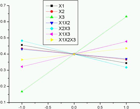
Figure 1. Effects of the parameters on the cost
|
Costs and the parameters |
|
|
|
Tests |
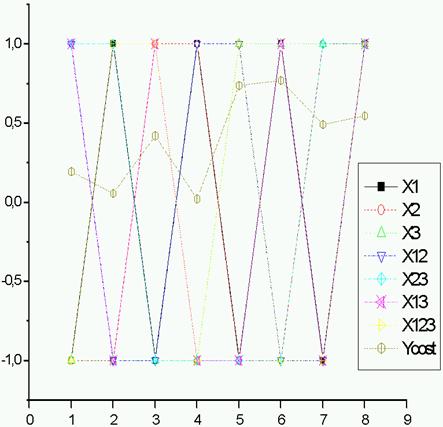
Figure 2. Influence N, Pm and Pc over the cost (Taguchi method)
The test No 6 (figure 2) is the best compared to the other tests, and with the best genetic operators (Pc =1.0, Pm = 0.001, N = 60) his cost is the best cost (5997.418).
Conclusion
In this work, we applied TPGA to the optimisation of the standard IEEE 118-bus model system. The obtained results were satisfactory. However in order to further the optimisation we used the experimental design method (Taguchi method). This allowed us to investigate the influences of the three parameters (Pc,Pm,N) that affect the outputs (cost function), The antagonism of the N effects upon the cost. This led us to a best solution which is the test number 6 as the best optimum compromise solution.
References
[1] Fletcher R., Practical Methods of Optimisation, John Willey & Sons, 1986.
[2] Rahli M., Ph.D. Thesis: Applied Linear and Nonlinear Programming to Economic Dispatch, Electrical Institute, USTO, Oran, Algeria, 1996.
[3] Stagg G. W. and E1 Abiadh A. H., Computer Methods in Power System Analysis, McGraw-Hill Book Company, New York, 1968.
[4] Himmelblau D.M., Applied Non Linear Programming, McGraw-Hill, New York, 1972.
[5] Younes M., Rahli M. and Koridak A., Dispatching Economique par l’Intelligence Artificielle, Proceeding ICEL’2005, U.S.T. Oran, Vol. 02, p. 16-21, November 13-15, 2005, Algeria.
[6] Holand, J. H., Adaptation in Natural and Artificial Systems, The University of Michigan Press, Ann Arbor, USA, 1975.
[7] Goldberg D. E., Genetic Algorithms in Search, Optimization and Machine Learning, Addison Wesley Publishing Company, USA, 1989.
[8] Lai L., Ma J. T., Yokoma R., Zhao M., Improved genetic algorithms for optimal power flow under both normal and contingent operation states, Electrical Power & Energy System, 19(5), p. 287-292, 1997.
[9] Chen B. S., Cheng Y. M., Lee C. H., A Genetic Approach to Mixed H2/H00 Optimal PID Control, IEEE Control System, p. 551-59, 1995.
[10] Younes M., Rahli M., Koridak H., La Répartition Optimale des puissances en utilisant l’algorithme génétique, ICEEE’2004, Laghouat, April 24-26, 2004, Algeria.
[11] Lin W. M., Cheng F. S., Tsay M. T., An improved tabu search for economic dispatch with multiple minima, IEEE Transactions on Power Systems, 17(1), p. 108-112, 2002.
[12] Sinha N., Chakrabarti R., Chattopadhyay P. K., Evolutionary programming techniques for economic load dispatch, IEEE Transactions on Evolutionary Computation, 7(1), p. 83-94, 2003.
[13] Park J. B., Lee K. S., Shin J. R., Lee K. Y., A particle swarm optimization for economic dispatch with nonsmooth cost functions, IEEE Transactions on Power Systems, 20(1), p. 34-42, 2005.
[14] Younes M., Rahli M., Koridak H., Genetic/Evolutionary Algorithms and Application to Power Systems, PCSE’05, O. Univ. El Bouaghi, May 9-11, 2005, Algeria.
[15] Benoist D., Tourbier Y., Germain-Peat S., worker: Experimental design: construction and analyzes. TCE & Doc. Lavoisier, Paris, 1994.
[16] Fowlkesand W.Y., Creveling C. M., Engineering Methods for Robust Product Design: Using Taguchi Methods in Technology and Product Development, Reading, MA, Addison-Wesley, 1995.
[17] Hedayat A. S., Sloane N. J. A., Stufken J., Orthogonal Arrays: Theory and Applications, Springer-Verlag, New York, 1999.
[18] Tanaka T., Optimization of Shaft Spline Teeth Design (in Japanese), Journal of Quality Engineering Society, Quality Engineering Society, 10(3) p. 80-84, 2002.
[19] Kumar S., & al, Quality improvements through design of experiments: a case study, Quality Engineering, 12(3), p. 407-16, 2000.
[20] Rowlands H., Antony J., Knowles G., An application of experimental design for process optimisation, The TQM Magazine, 12(2), p. 78-83, 2000.
[21] Roy R., Design of Experiments Using the Taguchi Approach, Wiley, New York, 2001.
[22] Berger P. D., Experimental Design, Duxbury Thomson Learning, 2002.
[23] Paris A., Târcolea C., Taguchi Applications on Manufacturing Systems, International Conference on Manufacturing Systems, Politehnica University Bucharest, p. 459-463, 2004.
[24] Tsui K. L., Modeling and Analysis of Dynamic Robust Design Experiments, IIE Transactions, 31, p. 1113-1122, 1999.
[25] Sanchez S. M., Robust Design: Seeking the Best of All Possible Worlds, Proceeding of the 2000 Winter Simulation Conference, p. 69-76, 2000.
[26] Anderson M. J., Kraber S. L., Using Design of Experiments to Make Processes More Robust to Environmental and Input Variations, Paint and Coating Industry, p. 1-7, 2002.
[27] Antony J., Simultaneous optimization of multiple quality characteristics in manufacturing processes using Taguchi’s quality loss function, International Journal of Advanced Manufacturing Technologies, 17, 134-8, 2001.
Short CV’s
Mimoun YOUNES was born in 1965 in Sidi Belabbes, Algeria. He received his BS degree in electrical engineering from the Electrical Engineering Institute of The University of Sidi Belabbes (Algeria) in 1990, the MS degree from the Electrical Engineering Institute of the University of Sidi Belabbes (Algeria) in 2003. He is currently Professor of electrical engineering at the University of Sidi Belabbes (Algeria). His research interests include operations, planning and economics of electric energy systems, as well as optimization theory and its applications.
Mostefa RAHLI was born in 1949 in Mocta Douz, Mascara, Algeria. He received his BS degree in electrical engineering from the Electrical Engineering Institute of the University of Sciences and Technology of Oran (USTO) in 1979, the MS degree from the Electrical Engineering Institute of the University of Sciences and Technology of Oran (USTO) in 1985, and the PhD degree from the Electrical Engineering Institute of the University of Sciences and Technology of Oran (USTO) in 1996. From 1987 to 1991, he was a visiting professor at the University of Liege (Monteore's Electrical Institute) Liege (Belgium) where he worked on Power Systems Analysis under tutee of Professors Pol PIROTTE and Jean Louis LILIEN. He is currently Professor of electrical engineering at The University of Sciences and Technology of Oran (USTO), Oran, Algeria. His research interests include operations, planning and economics of electric energy systems, as well as optimization theory and its applications.