General Linear Methods
Abraham OCHOCHE
Department of Mathematics / Computer Science, Federal University of Technology, Minna, Nigeria
Abstract
General linear methods were originally introduced as a platform for the unified study of consistency, stability and convergence for a large class of numerical methods for ordinary differential equations. Because general linear methods are not well known even though they have been in existence for about forty years, we here attempt an introduction of these very useful and interesting methods that is suddenly generating so much interest in the scientific world. We introduce the use of this formulation and discuss the meaning of consistency, stability convergence and order for these methods. We also demonstrate how some traditional methods can be represented as general linear methods.
Keywords
General linear methods, Differential equations
1. Introduction
Ordinary differential equations arise frequently in the study of physical systems. Unfortunately, many cannot be solved exactly. This is why the ability to numerically approximate these methods is so important [[1]].
General linear methods were originally proposed [[2]] as a unifying framework for studying stability, consistency, and convergence for a wide variety of methods. Not only does their formulation includes both Runge-Kutta and linear multistep methods in a natural way, but also allows for various generalizations of these methods proposed by a number of authors [[3], [4], [5]]. In section 2, we present a summary of the evolution of numerical methods; we also give an overview of general linear methods. In section 3, we will review the basic definitions of stability, consistency and convergence and indicate the relationship between them. In section 4, we discuss the concept of order for general linear methods and show through some examples how it can be analyzed in practice. In section 5, we introduce the framework for these methods now in common use and show how a number of special method types can be represented within this framework.
2. General linear methods
When Euler proposed his method in 1768 [1], it represented the simplest method available to numerically approximate the solution of an ordinary differential equation.
In the formulation of this method we note that [[6]]:
(i) yn+1 depends explicitly on yn but on no earlier of yn, yn-1, …
(ii) The function f is evaluated only once in the step from the computation of yn to the computation of yn+1;
(iii) Only the function f itself is used rather than f2, f3, … say which yield values of y′′(x), y′′′(x),…, in terms of y(x) or of f′′ (the Jacobian of f), f′′, …
Euler method is both one-step and multi-step, and this fact together with the stability requirements, can mean that h has to be chosen to be very small and as noted in, “the method of Euler is ideal as an object of theoretical study but unsatisfactory as a means of obtaining accurate results.” [6]. Due to the low accuracy and poor stability behaviour, generalizations have been made to the method of Euler.
The most important generalizations of the Euler method [6] are:
(a) The use of formulae that violate (i). That is, yn+1 depends on yn-1, …, yn-k(k ≥1) as well as on yn. These methods are known as linear multistep methods.
(b) The use of formulae that violates (ii). That is more than one evaluation of f is involved in a formula for yn+1. These methods are known as Runge-Kutta methods.
(c) The use of formulae that violate (iii). For example, expressions for y′′(x), y′′′(x),… may be used along with an expression for y′(x). The Taylor series method.
The notable generalizations of the Euler method are (a) and (b). These two traditional classes of numerical methods for ordinary differential equations have always been studied separately. For linear multistep methods, the difficult questions have always been associated with the stability of the sequence of approximations produced whereas accuracy question are relatively simple. For Runge-Kutta methods, stability is a very straightforward matter but accuracy questions are exceedingly complicated. A good number of methods have been introduced that fall somewhere in-between these two traditional methods, for which the existing theories proved, to some extent, inadequate [[7]].
General linear methods were introduced [2] to provide a unifying theory of the basic questions of consistency, stability and convergence. Later they were used as a framework for studying accuracy questions and later the phenomena associated with nonlinear convergence. They combine the multi-stage nature of Runge-Kutta methods with the notion of passing more than one piece of information between steps that is used in linear multistep methods. Their discovery opened the possibility of obtaining essentially new methods that were neither Runge-Kutta nor linear multistep methods would exist which are practical and have advantages over the traditional methods.
These extremely broad class of methods, besides containing Runge-Kutta and linear multistep methods as special cases also contain hybrid methods, cyclic composite linear multistep methods and pseudo Runge-Kutta methods [1, [8]].
A general linear method used for the numerical solution of an autonomous system of ordinary differential equations:
y′(x) = f(y(x)), x ![]() [x0,
[x0, ![]() ], y : [x0,
], y : [x0,
![]() ]
→
]
→![]() m,
f(y(x)) :
m,
f(y(x)) : ![]() m
→
m
→![]() m
m
where m is the dimensionality of the system, is both multistage and multivalue. We denote the internal stage values of step number n by Y1[n], Y2[n], …, Ys[n] (s is the internal stage number) and the derivatives evaluated at these steps by f(Y1[n]), f(Y2[n]), …, f(Ys[n]).
At the start of step number n, r quantities denoted by y1[n-1], y2[n-1], …, ys[n-1] are available from approximations computed in step n-1.
Corresponding quantities y1[n], y2[n], …, ys[n] are evaluated in the step number n. for compactness of notation, we introduce vectors Y[n], f(Y[n]), y[n-1] and y[n] given by:

If h denotes the stepsize, then the quantities imported into and evaluated in step number n are related by:
Y[n] = h(A ![]() Im)
f(Y[n]) + (U
Im)
f(Y[n]) + (U ![]() Im) y[n-1]
Im) y[n-1]
y[n] = h(B ![]() Im)
f(Y[n]) + (V
Im)
f(Y[n]) + (V ![]() Im) y[n-1],
where n = 1, 2, …, N
Im) y[n-1],
where n = 1, 2, …, N
For ease of representation, the Kronecker product with Im will be removed. The method is then:
Y[n] = h A f(Y[n]) + U y[n-1]
y[n] = h B f(Y[n]) + V y[n-1], where n = 1, 2, …, N
In [6], the notation was introduced by which a general linear method is represented by a partitioned (s+r) x (s+r)
![]() .
.
Hence, general linear methods take the form:

where r is the number of pieces of information that is passed from step to step and s is the number of internal stages.
The structure of the leading coefficient matrix A, determines the implementation costs of these methods (similar to that of the A matrix in Runge-Kutta methods). General linear methods can also borrow popularized names used in Runge-Kutta theory such as “Diagonally Implicit”, when the A matrix is lower triangular, “Singly Implicit”, when the A matrix has a single eigenvalue and “Implicit”, when the A matrix is full. The V matrix determines the stability of these methods and it is required that V be power bounded [[9]]. The U matrix gives the weights that need to be assigned to y(xn), y′(xn) and y′′ (xn).
3. Preconsistency, consistency, stability and convergence
As in the case of linear multistep methods, a general linear method needs to be consistent and stable in order to give meaningful results [1, [10]]. The quantities passed from step to step could be seen as representing approximations to the solution y(x), the scaled derivative hy′(x) values, or arbitrary linear combinations of such quantities, therefore, we can only define consistency in a rather general manner [10].
Let u and v be two m dimensional vectors referred to as the “preconsistency” and “consistency” vectors, respectively. These vectors imply that yr[n] is intended to approximate ur y (xn) + h vr y′ (xn). If e is an r dimensional vector of 1’s, then the full preconsistency and consistency conditions are given by:
V u = u, U u = e, Be + Vv = u + v, Ae + Uv = c
If equation (2) is satisfied, then at the very least, a method should be able to solve the trivial initial value problem y′(x) = 0, y(0) = a, exactly both at the beginning and at the end of each step.
Stability can be defined, as a generalization of the definition of stability for linear multistep methods; as a requirement that the matrix V is power bounded.
As with linear multistep methods, it is known that stability and consistency are necessary and sufficient conditions for convergence [2]. Without being too formal, we can describe convergence as “the ability of a numerical method to produce approximations that converge in the limit as the number of steps tends to infinity (as the stepsize converges to zero in an appropriate manner) to the exact solution with the r values scaled according to the components of the preconsistency vector” [10].
4. Order of general linear methods
As for all multi-value methods, some sort of starting procedure is
required to obtain an initial vector, y[0], from the initial
value y0 before the first step can be carried out. If we let ![]() be the
internal stages, the starting procedure can be defined as:
be the
internal stages, the starting procedure can be defined as:
![]() =
h S11 f (
=
h S11 f (![]() ) + S12y0
) + S12y0
y[0] = h S21 f(![]() ) + S22y0
) + S22y0
This can be written as the (![]() + r) x (
+ r) x (![]() +1)
+1) ![]() partitioned tableau:
partitioned tableau:

where ![]() is the number
of internal stages and r is the number of initial approximations
required. Preconsistency demands that S22 = u and S12
=
is the number
of internal stages and r is the number of initial approximations
required. Preconsistency demands that S22 = u and S12
= ![]() .
Generally, if a method is of order p each of the r components of y[0]
will be of order at least p.
.
Generally, if a method is of order p each of the r components of y[0]
will be of order at least p.
We can now define the order of a method in relation to a starting method S. Applying the starting method, S, to a problem, followed by one step of the method M the result is M · S. The operator E represents the exact solution shifted one step forward. If it were possible to take one step forward in time using E then applying the starting method, the result would be S · E. It is obvious from the figure below, that a method is said to be of order p if the difference between these two approximations is o(h p+1) i.e. M · S - S · E = o(h p+1). We must note that since it is the first component of the solution that approximates y(xn), this would imply that it is only the first component that is required to be O(h p+1) to have a method of order p.
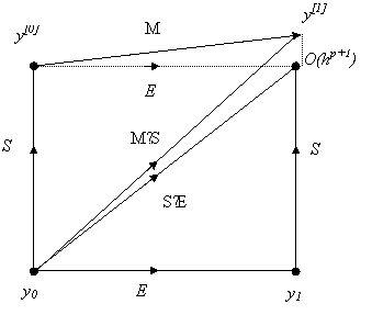
Figure1. The order of a general linear method
5. Representation framework
In order for general linear methods to unify the somewhat opposing traditional methods, it must be possible to represent these traditional methods using the partitioned M matrix above.
As shown in [10, [11], [12]], Runge-Kutta methods are very simple to rewrite as general linear methods. The A matrix of the general linear method, is the same as the A matrix of the Runge-Kutta method. The B matrix is bT where b is the vector of weights of the Runge-Kutta method. Assuming the input vector is an approximation to y(xn-1), the U matrix is simply e, a vector of 1’s. The V matrix consists only of the number 1. It is thus written as:

For instance, the classical fourth-order Runge-Kutta method with Butcher tableau

has a general linear form in terms of the matrix

Runge-Kutta methods always have r = 1, since only one quantity is passed from one step to the next.
Linear multi-step methods have a general linear form given by the matrix:

The Adams-Bashforth method:
yn = yn-1 + h [3 f(yn-1) - f(yn-2)] / 2
has the general linear formulation thus

The linear multistep methods have s = 1 because the function f is evaluated only once in each step.
Predictor-Corrector methods:
y* = yn-1 + h k Ski=1 β*i f (yn-1)
y* = yn-1 + h β0if (y*n) + h Ski=1 βi f (yn-1)
can be implemented either as a PEC (Predict Evaluate Correct) or PECE (Predict Evaluate Correct Evaluate) schemes. A PEC method can be expressed in genera linear form as

whereas a PECE method can be written in general linear form as:

The second order two-step Adams-Bashforth and the second order one-step Adams-Moulton pair of methods put together as a predictor-corrector pair:
yn = yn-1 + h [3 f(tn, yn) - f(tn-1, yn-1)] / 2
yn+1 = yn + h [f(tn+1, y[0]n+1) - f(tn, yn)] / 2
in PECE mode can be expressed in general linear form as:

6. Conclusions
General linear methods were introduced to provide a unifying framework for the traditional methods. We presented an introductory view on general linear methods, and we have also demonstrated its unifying capabilities by demonstrating how the traditional methods can be expressed as general linear method.
7. Special acknowledgement
The author wishes to acknowledge the immense contributions and cooperation’s received from Prof. John C. Butcher, of the University of Auckland, New Zealand, as well as Dr. Nicolette Rattenbury, of the Manchester Metropolitan University.
References