Improving the Modified Euler Method

Abraham OCHOCHE

Mathematics/Computer Science Department, Federal University of Technology Minna, Nigeria

abochoche@yahoo.com

Abstract

The purpose of this paper was to propose an improved approximation technique for the computation of the numerical solutions of initial value problems (IVP). The method we have improved upon is the Modified Euler method. By the simple improvement we effected we were able to obtain a much better performance by our Improved Modified Euler (IME) method which was shown to also be of order two.

Keywords

Differential equations, Initial Value Problem, Modified Euler, Improved

Introduction

The purpose of this paper is to propose a modified approximation technique for the computation of the numerical solutions of initial value problems (IVP). The method we are attempting to improve upon is the Modified Euler method.

Differential equations are one of the most important mathematical tools used in modeling problems in physical sciences. Historically, differential equations (DE) have originated in chemistry, physics and engineering. More recently, they have also arisen in medicine, biology, anthropology, and the like. Ordinary differential equations arise frequently in the study of physical systems. Unfortunately, many cannot be solved exactly. This is why the ability to numerically approximate these methods is so important [12].

Numerical solution of ODEs is the most important technique ever developed in continuous time dynamics. Since most ODEs are not soluble analytically, numerical integration is the only way to obtain information about the trajectory. Many different methods have been proposed and used in an attempt to solve accurately, various types of ODEs All these, discretise the differential system, to produce a difference equation or map.

The methods, obtain different maps from the same equation, but they have the same aim; that the dynamics of the maps, should correspond closely, to the dynamics of the differential equation [8].

With the advent of computers, numerical methods are now an increasingly attractive and efficient way to obtain approximate solutions to differential equations that had hitherto proved difficult, even impossible to solve analytically.

An Historical Perspective

When Euler proposed his method [1],

yn+1 = yn + hk1

(1)

where k₁ = f(x_n, y_n)

            It represented the simplest method available to numerically approximate the solution of an ordinary differential equation.

In the formulation of equation (1) we note that [4]:

· y_n+1depends explicitly on y_n but on no earlier of y_n, y_n-1, …

· the function f is evaluated only once in the step from the computation of y_n to the computation of y_n+1;

· only the function f itself is used rather than f₂, f₃, … say which yield values of y′′(x), y′′′(x), in terms of y(x) or of f′ (the Jacobian of f), f′′, …

Euler method is both one-step and multi-step, and this fact together with the stability requirements, can mean that h has to be chosen to be very small and as noted in [4], “the method of Euler is ideal as an object of theoretical study but unsatisfactory as a means of obtaining accurate results”. Due to the low accuracy and poor stability behavior, generalizations have been made to the method of Euler.

The most important generalizations of equation (1) are:

(a) The use of formulae that violate (i). That is, y_n+1 depends on y_n-1, …, y_n-k (k ≥ 1) as well as on y_n These methods are known as linear multistep methods;

(b) The use of formulae that violates (ii). That is more than one evaluation of f is involved in a formula for y_n+1. These methods are known as Runge-Kutta methods (and include methods such as mid-point quadrature rule and trapezoidal method).

(c) The use of formulae that violate (iii). For example, expressions for y′′(x), y′′′(x), … may be used along with an expression for y′(x). The Taylor series method is an example of such a method [4].

The notable generalizations of the Euler method are (a) and (b). As Runge [2] observed, Euler’s method give rise to a rather inefficient approximation of the integral by the area of a rectangle of height f(x₀) (see Fig. 1(a)).

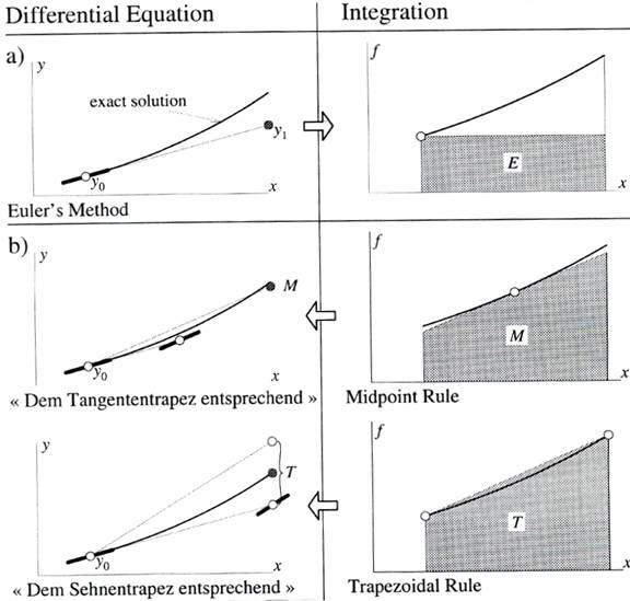
Figure 1. Runge’s motivation culled from [9]

Therefore, he stated that “it is already much better” to extend the Midpoint rule:

yn+1 = yn + hf(xn + h/2, y(xn + h/2))

(2)

and the Trapezoidal  rule:

yn+1 = yn + h/2(f(xn,yn) + f(xn+1,yn+1))

(3)

to differential equations (see Fig. 1(b))by inserting the forward Euler step for the missing y-values to obtain the Modified Euler method [9]:

yn+1 = yn +hf(x0 + h/2, y0 + h/2f(xn, yn))

(4)

which we can rewrite as:

y_n+1 = y_n + hk₂

where

k₁ = f(x_n, y_n) and k₂ = f(x_n + h/2, y_n +k₁h/2)

The Improved Euler method:

yn+1 = yn +h/2(f(x0,y0) + f(xn + h, yn + hf(xn,yn)))

(5)

which we can also rewrite as:

y_n+1 = y_n + h/2(k₁ + k₂)

where

k₁ = f(x_n,y_n), k₂ = f(x_n + h, y_n + hk₁)

respectively. These methods are both know to be of order 2.

Improving the Modified Euler’s Method

What we are attempting to achieve, is an improvement on the Modified Euler method.

We hope to achieve this, by inserting the forward Euler method, in place of in the inner function evaluation of the Modified Euler method thus:

yn+1 = yn + hf(xn + h/2, yn + h/2·f(xn, yn +hf(xn,yn)))

(6)

            We can go on to rewrite it as:

yn+1 = yn + hk2

(7)

with: k₁ = f(x_n,y_n), k₂ = f(x_n +h/2, y_n + h/2·f(x_n, y_n + hk₁))

Order of the Proposed Method

In this section, we shall attempt to obtain the order of our new method. This we hope to achieve by first carrying out a Taylor series expansion of the k_is (i = 1,2) and then of y_n+1 as well. We will then proceed to equate as many terms as possible in both expansions. If we are able to equate terms up to and including O(h^p), then the method is of order p [5].

We now proceed to expand the k_is (i = 1,2) in turn by Taylor’s theorem [ 11]:

f(x+m, y+n) = f(x,y) + Df(x,y) + 1/2·D^2f(x,y) + … + 1/n! · D^nf(x,y)

(8)

where:

D = m(∂/∂x) + n(∂/∂y) and D^nf(x,y) = [m(∂/∂x) + n(∂/∂y)]^nf(x,y) k1 = f(x,y) = f k2 = f + h/2·fx + h/2·f(xn,yn + hk1)fy + h^2/4·fxx + h^2/2·f(xn, yn + hk1)fxy +       + h^2/4·(f(xn, yn + hk1))^2fyy + h^3/8·fxxx + 3/8h^3f(xn, yn + hk1)fwwy +       + 3/8h^3(f(xn,yn + hk1))^2fxyy + 1/8h^3 (f(xn, yn + hk1))^3 + O(h^4)

(9)

Without loss of generality, equation (9) can be written as:

k2 = f + h/2·fx + h/2·ffy + h^2/4·fxx + h^2/2·ffxy + h^2/4·f^2fyy + h^3/8·fxxx + 3/8·h^3ffwwy        + 3/8·h^3f^2fxyy + 1/8·h^3f^3fyyy + O(h^4)

(10)

Collecting like terms in powers of h:

k₂ = f + h/2( f_x+ ff_y) + 1/4·h²(f_xx + 2ff_xy + f²f_yy) + 1/8·h³(f_xxx + 3ff_xxy3f²f_xyy + f³f_yyy) +

       + O(h⁴)

Adopting the notation in [7], [10]:

Set: F = f_x + ff, G = f_xx2ff_xy + f²f_yyy, H = f_xxx + 3ff_xxy + 3f²f_xyy + f³f_yyy

Þ k₂ = f + 1/2·hF + 1/4·h²G + 1/8·h³H + O(h⁴)

When our derived expressions for and are substituted into equation (7) we obtain:

yn+1 = yn + hf +1/2·h^2F + 1/4·h^2G + 1/8·h^3H

(11)

The Taylor series for y_n+1 is given by:

yn+1 = yn + hy^′n + 1/2·h^2y^′′n + 1/3!·h^2 y^′′′n + O(h^4)

(12)

Next, we need to express the derivatives in equation (12) in terms of f(x_n,y_n) and from [7], [10] they are:

y^′ = f, y^′′ = F, y^′′′ = G + Ffy

(13)

Slotting (13) into equation (12) we obtain:

yn+1 = yn + hf + 1/2·h^2F + 1/3!·h^2G + 1/3! ·Ffy + O(h^4)

(14)

On comparing the terms in equations (11) and (14) we immediately see that they agree up to and including O(h²) only. From our assertion at the beginning of this section, we can conclude that our new method, is of order 2 i.e. the local error is O(h³) [9].

Numerical Experiments

            In this section, we present the solution of some initial value problems using the new method which we shall henceforth refer to as Improved Modified Euler (IME) method. We present the results along with those obtained using the well known Modified Euler (ME) method. Both problems were solved using a constant steplenght (h) of 0.1 we are hoping for an improved performance.

            The problems we will be working with are:

i. y′ = x + y, y(0) = 1

ii. Problem A1 (the negative exponential) in the DETest problem set [3]: y′ = - y, y(0) = 1

The results are presented in Figures 2 and 3 below:

Figure 2. Comparing the Modified Euler (ME), and our Improved Modified Euler (IME) method for problem i

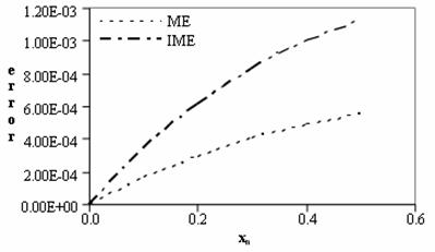
Figure 3. Comparing the Modified Euler (ME) method and our Improved Modified Euler (IME) method for problem ii

Discussion

We can observe from Figures 2 and 3, that the our IME method does not only hold its own against the ME method it actually out performs it with regards to the non-autonomous problem i. Unfortunately however the IME method did not fare so well in comparison with the ME method for the second problem which is an autonomous IVP.

Conclusion

In this paper, we have made an attempt at improving upon the already existing Modified Euler method. We have also gone on to show that our Improved Modified Euler method is also of order 2. We have also carried out some numerical experiments to compare our IME method with the Modified Euler method, and we have been able to obtain an improved performance. We were hampered from carrying out more extensive experiments due to non-availability of necessary hardware and software.

References

[1]     Euler H., Institutiones calculi integralis. Volumen Primum (1768), Opera Omnia, Vol. XI, B. G. Teubneri Lipsiae et Berolini MCMXIII.

[2]     Runge C., Ueber die numerische Auflösung von differentialgleichungen, Math Ann 46, 1895.

[3]     Hull T. E. et al, Comparing numerical methods for ordinary differential equations, SIAM J Numer Anal 9, 1972.

[4]     Butcher J. C., General linera methods: A survey, Appl Numer Math 1, 1985.

[5]     Fatunla S. O., Numerical methods for initial value problems in ordinary differential equations, Academy Press Inc. (London) Ltd.

[6]     Kendall E. A., An introduction to numerical analysis (second edition), John Wiley and Sons, 1989.

[7]     Lambert J. D., Numerical methods for ordinary differential equations, John Wiley and Sons, USA, 1991.

[8]     Julyan E. H. C., Piro O., The dynamics of Runge-Kutta methods, Int’l J Bifur and Chaos  2, 1992.

[9]     Butcher, J. C. and Wanner, G., Ruge-Kutta methods: some historical notes, Appl Numer Math 22, 1996.

[10]   Adewale I. K., A new five-stage Runge-Kutta method for initial value problems, M Tech Dissertation, Federal University of Technology, Minna, Nigeria, 1998.

[11]   Abraham O., A fifth-order six stage explicit Runge-Kutta method for the solution of initial value problems, M. Tech Dissertation, Federal University of Technology, Minna, Nigeria, 2004.

[12]   Rattenbury N., Almost Runge-Kutta methods for stiff and non-staiff problems, Ph.D Dissertation, The University of Auckland, New Zealand, 2005.