Neural Network Control of CSTR for Reversible Reaction Using Reverence Model Approach
Dauda Olurotimi ARAROMI1, Tinuade Jolaade AFOLABI1, Duncan ALOKO2
1Department of Chemical Engineering ,Ladoke Akintola University of Technology, Ogbomoso, P.M.B 4000,Oyo State, Nigeria
2Department of Chemical Engineering, Federal University of Technology, P.M.B 65, Minna. Niger State, Nigeria
aradachem@yahoo.com, tinuadeafolabi@yahoo.com, alokoduncan@yahoo.com
Abstract
In this work, non-linear control of CSTR for reversible reaction is carried out using Neural Network as design tool. The Model Reverence approach in used to design ANN controller. The idea is to have a control system that will be able to achieve improvement in the level of conversion and to be able to track set point change and reject load disturbance. We use PID control scheme as benchmark to study the performance of the controller. The comparison shows that ANN controller out perform PID in the extreme range of non-linearity.
This paper represents a preliminary effort to design a simplified neutral network control scheme for a class of non-linear process. Future works will involve further investigation of the effectiveness of thin approach for the real industrial chemical process
Keyword
Neural Network, Model Reverence, Model identification
Introduction
With the advent of high-speed computer system, there is more increase interest in the study of non-linear system. The need for this interest is born out of the fact that most industrial process is inherently non-linear and reasons, which include, higher quality specification, improvement in productivity, tighter regulations on environment, and demand for operating safety and high quest for economic profitability have called for to operate system over the boundary of a wide range of operating conditions and often near the boundary of a admissible region. It is nonlinear system that is able to describe the dynamic behavior under these conditions (Rolf Findeisen et al, 2003).
Neural network technology has received much attention in the field of chemical process control, this is because of inherently non-linear nature of most of the processes and neural network have great capability in solving complex nonlinear mathematical problem (Junghui and Titen-chu, 2004).
Neural networks have shown great progress in identification of nonlinear system, which is due to increase in cheap computing power and certain powerful theoretical algorithms (Cybenko, 1989; Lippman, 1987; Rumelhart and Mecelland; 1986).
Application of ANNs to non-linear process control have attracted a rapidly growing interest in the recent time (Willis et al, 199, Hunt et. al, 1992) several approaches have been used to train ANN to model either the process behavior or its inverse and subsequently used within conventional model based control schemes including model based predictive control, internal model control, adaptive control and feed forward control (Hunt and Sbarbaro, 1992; Barto, Sutton and Anderson, 1983).
It has been used effectively in design of model-based control, such as the direct and indirect neural network model based control (Psichogios, 1991), nonlinear internal control (Nahas etal, 1992), and recurrent neural network model control (Nikolaou and Hanagandi, 1990). Except that the nonlinear iterative algorithm of the control design in computational demand, the control performance based on this strategy is very satisfactory, its implementation is very realistic for control of slow dynamic process.
About 95% industrial control loops are still based on proportional integral derivative (PID.) controller; this is because of simplicity in its structure, robustness in its operation and ease of comprehension of its principle (Aston and Hagglund, 1995). However, most of the industrial PID controllers deteriorate in performance when they are dealing with highly nonlinear process.
Several self- turning scheme have been proposed in the past to arrest the deteriorative performance in the face of nonlinearity ,however little achievement have been made because most of these schemes were designed on the assumption that controller together with process model are operating in a linear region. One major draw back in the operation of these schemes is that whenever there is a change in operating condition. It will require manual check to confirm if the model represents real plant because control design is totally based on reliable model.
Gain scheduling is one of the approaches used for PID control design to capture nonlinear behavior of real plant. In this many linearized models are obtained around different operating systems and a set of predefined linear controllers are selected. Each controller is turned for a specific operating region.
In the work of Fuli et al (1984), neural network with pole placement design method was proposed. In this method, the plant was linearized at a particular operating point. Then linear neural network was then developed on-line to mimic the linear dynamic behavior of process at this operating point to which multilayer feed forward neural network was used to identify nonlinear and use this as a measured disturbance. Pole placement was used as feedback control and the multi layered feed forward neural network as feed forward control to eliminate the nonlinear disturbance. Junhui and Then Chih (2004) proposed an on line updated PID algorithm. This combined the general minimum variance (GMV) control law with instantaneous extraction of characteristics linearized neural network.
In this work, nonlinear control of CSTR for reversible reaction is done to bring about 100% conversions and to suppress backward reaction. Two control schemes, PID control and ANN model reference based control are considered. The two are studied for setup change, disturbance effect and model - plant mismatch.
In the sections that follow, we will have these arrangements, reactor dynamic modeling for reversible reaction, PID control design, followed by neural network controller design, results are discussed concurrently conclusion is then made.
Reactor dynamic modeling
To design a chemical reactor with its associated control equipment, it is necessary to study dynamic behaviour of the system. The modeling equation governing the dynamic of a cooling continuously stirred tank reaction (CSTR) with a first order reversible reaction:
![]()
can be derived from the mass and energy balances equation of the reactor (Aris R., and Amundson N. R., 1958).
Figure 1. CSTR with cooling system
With the assumption that the feed is free of product B, the balance equation for an ideal CSTR can be written as:
|
|
(1) |
|
|
(2) |

The effect of temperature on the reaction rate k is usually found to be exponential:
|
|
(3) |
where k0 is a pre-exponential (or Arrhenuis ) factor.
To model the rate of heat transfer to cooling coil or jacket it is assumed that coolant dynamic is negligible on the premise that cooling flow rate is fast compared to feed flow rate so, the balanced equation for the cooling jacket or coil is:
|
UA(T - TC) = Fcρc(Tcin - Tco) |
(4) |
where the following notations were used: CA = concentration of reactant A; CP = mixture heat capacity; CPC = coolant heat capacity; CAin = feed concentration of A; Ej = activation energies of reactions; Fc = cooling area; ΔHR = heat of reaction; ki = velocity constants; U = Heat transfer coefficient; Fa = coolant flow rate; R = gas constant; TC = coolant temperature; Tcin = coolant input and output temperature; V = volume of reactor; T = time; ρ = density; ρc = coolant density; A = cooling area.
The following parameters are used to simulate the reactor dynamics.
|
Value of system parameter |
Steady state |
||
|
CAin = 1000mol |
CBin = 0.0 |
G = 5.24103 |
Tin = 427k |
|
V = 100litre |
ΔHR =20920 |
C2 = 1.32∙106 |
Tco = 300K |
|
ρ = 1.5∙104 kg/m3 |
Cp = 4292 |
E1 = 4/840 |
R = 8.2314 |
|
ρc = 1000 kg/m 3 |
Cpc = 4184 |
E2 = 62760 |
|
PID controller
The three term proportional integral derivative PID controller account for more than 95% of installed automatic feedback controller (Junghui and Tien-Chih, 2004). PID controller gave optimal control for 1st order system without and delays. There are three classes of PID in this work; the class chosen has the generic form:
|
|
(6) |
The variable e(t) represents the tracking error, the difference between the desired value (r) and the actual output (y). This error signal will be used by PID controller. PID will take appropriate action according to the law and pass the signal (u) to the plant to adjust the appropriate manipulated variable.
Optimal Models for Model Reference Control
Reference model is a desired forward dynamic response .In model reference control; ANN controller is designed to make the process output behaves similar to the reference model. In this work, we consider optimal model for our design. Model is said to be optimal with respect to cost criteria J, if the cost is lowest when using that model. The most common cost criteria are integrals of the absolute error (IAE), the squared error (ISE), the time weighted error (ITAE) and the time weighted squared error (ITESE). The IAE and ISE cost criteria weight the initial values of the error more than the later value while the time weighted criteria such as the ITAE criteria weight the later values of the error more. Minimizing the integral constraint tries to keep the error small in general sense. In this work, we used ITAE as our cost criterion.
The nth order model considered has the form:
|
|
(7) |
For some nth order (monic) denominator poly nominal D is given by
|
|
(8) |
We have this polynomial expressed in terms of the natural frequency; ω0. Bandwidth, which measure the effectiveness of dynamic polynomial of system of the can be adjusted through this parameter. Here the numerator is constant hence relative degree of the model is equal to the order of the denominator. Optimization computation using a Monte-Carlo method of optimization called a random neighborhood search (RSN) (Franklin, et al; 1990) involved searching for the best set of coefficient to satisfy the given cost criteria that will provide zero steady state error.
The search began with a stable denominator, and ω0. = 1. The system was simulated and the cost associated with that polynomial was computed. A polynomial with coefficient near the previous (randomly chosen) was obtained and the system re simulated and the cost recalculated. This process was continued until the set criteria were met.
Network Structure and Representation
In this work, the type of network structure employed is multi layer, layer perception (MLP),which is one type of feed forward network. Neural. A MLP consists of an input layer, several hidden layers, and an output layer.
Node i, also called a neuron, in a MLP network is shown in Fig. 2. It includes a summer and a nonlinear activation function g.
Figure 2. Single node in a MLP network
Input to the preceptor are individually weighted and summed. The preceptor computes the output as a function g of the sum. The activation energy, g in needed to introduce non-linear into the network. Thin makes multilayer network a powerful representation of nonlinear system. The output from the single node is computed by:
|
|
(9) |

Connecting several nodes in parallel and series, a MLP network is formed. A typical network is shown in Figure 3.
Figure 3. A multilayer perceptron network with one hidden layer; the same activation function g is used in both layers
The output, 1, 2, i y i= of the MLP network becomes:
|
|
(10) |

Training is the process of adjusting the weights. The training is intended to steadily adjust the connection weight in order to minimize the mean square error between target value output and predicted value output. Training usually begins with random values for the weights of NN. Then, the networks are supplied with a set of samples belonging to problem domain to modify the values of their weightThe weights are dynamically updated using back propagation leaning algorithm (Saerens & Soquet A., 1991). There are two moves before the weights are updated. In the first move (forward move) the outputs of all neurons are calculated by multiplying the input vector by the weights and the error is calculated for each of the output layer neuron. In the backward move, the error is passed through the network layer and the weight are updated according to the gradient steepest rule, so that the actual output of the MLP moves closer to the desire output. The difference between the target output and the computed output is known as error, this error is computed as:
|
ei(k) = T1(k) - yi(k) |
(11) |
The errors are back propagated through the layers and the weight adjustments are made. The formula for adjusting the weight is:
|
wij(k+1) = wij(k) + μei(k)xi(k) |
(12) |
where μ is learning rates, once the weights are adjusted the feed - forward process is repeated. The training is interned to gradually adjust the connection weight in order to minimize the mean square error. (MSE):
|
|
(13) |
where
· M: number of training data pattern
· N:- number of neurons in the output layer.
· Ti(k) = the target value of the output neurons for the given kth data pattern.
· Yi(k)- the prediction for the ith output neurons given the kth data pattern.
The main advantages of neural network are its ability to supply fast answers to a problem and its capability to generalize answers thus providing acceptable result for unknown samples (Cholamreza Zahedi et al, 2005).
ANN Controller Design
Model Reference Control
An illustration of model reference control is presented in figure 4. In the figure the network has two inputs, one of the inputs is difference between plant output and model reference output and second input is difference between model output and reference signal.
Both plant model and reference model are used to train the network. The resulting ANN model will serve as controller for the system. Fig.4 explains the model reference control system. ANN controller uses these to adjust its weights until the output of the plant looks similar to model reference output trajectory
ANN controller will have two input, error signal from reference model output, and plant output, the second error signal comes from difference between reference signal and plant output. The procedures involved in training the network are generation and validation of training data sets; preprocessing of data set and training and validation of network. To have good representation of the model, two data sets were generated from the system to train the network, one data set for validation and another one testing. Uniform random input signals, which span the upper and lower limit of operating range, were used to excite the system. This was done to enable network learn the nonlinear nature of the system. Before incorporating the network into the control scheme the networks was trained offline using the Gauss-Newton based Levenberg Marquardt algorithm (K. Leleberg 1944 and D. W. Marquardt 1963). The essence is to let the network learn the functional nonlinearities to a certain degree of accuracy before implementing into the controller, and thus can give faster online adaptation as need. In this study data sets for the training were obtained by carrying out simulation on the open loop of the system. 20,000 data sets were generated to train, validate and test the trained network.
Figure 4. Model Reference Control
The network considered was MLP with a single hidden layer. The activation function used in study is nonlinear sigmoid function in hidden layer and the linear function in the output layer. Neural network with large enough number of hidden neurons, which has continuous and differentiable transfer function can approximate any continuous function over a closed interval (Cybenko, 1989) .The numbers of nodes are initially fixed at small numbers, the number was increased in order to have a proper trained network. Satisfactory networks model were obtained when the sum of squared errors of the validation data set was satisfactorily small.
The first step in the design is plant identification; here data for the identification were generated by simulating CSTR model. The data generated was used to train the ANN. The type of training is supervised learning described in section 2.3 the network has 20 neurons in the hidden layers. The activation functions in the hidden layer are tan-sigmoid and the output layer in a linear function.
Simulation Result and Discussion
The open loop simulation of CSTR for reversible reaction is shown in figure 5. Here, the product concentration is plotted against time. The reaction considered was 1:1 mole ratio of reactant to product. For complete conversion, the curve is expected to reach maximum of 1mol/L for one mole reactant. This is not so because the reaction considered is a reversible reaction and there is backward reaction after a long period of time.
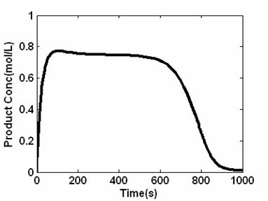
Figure 5. Product Concentration profile for open loop simulation of CSTR for reversible reaction
Figure 6 shows the temperature profile of the system; it is observed that the system is unstable because the temperature is infinitely increasing for the system.
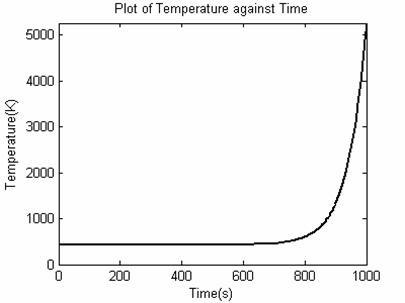
Figure 6.Temperature profile for open loop simulation of CSTR for reversible reaction
In order to bring the reaction to complete conversion and to prevent backward reaction, the flow rate of reactant was used as manipulated variable in the control design.
Figure 7 shows response for both ANN and PID controller. For PID controller, the controller setting that gave the best performance was found to be Kc = 3.15, Ki = 0.4 and Kd = 8. The response is not without of overshooting, which is very high and small inverse response. For the case of ANN the overshoot is very small but in both cases, they brought the reaction almost into complete conversion.
The next performance test involved a set point tracking problem the set point was allowed to change in random fashion. Figure 8 show the result obtained using the ANN reference model based control strategy. The system behavior shows perfect tracking with no overshoot although the system is somehow sluggish which may be accommodated for the system under consideration. The dotted line in fig 8 shows the performance of a PID controller. Overshoot is observed and settling time for the first set point is quite long. But for the subsequent set points PID response looks similar to ANN with small over shoot. The plots also show an unsymmetrical response of PID control for different set points, implying that the system behave nonlinearly for PID control.
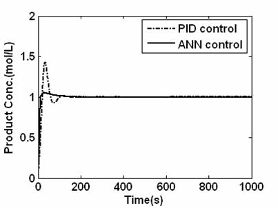
Figure 7. Closed loop response for the system under PID and ANN control

Figure 8. Closed loop responses for set point tracking for the system
We now examine the system response in the presence of external disturbance. The system was disturbed by introducing 10% change in reactant temperature. The response obtained for this disturbance is shown in figure 9, ANN controller was fast to arrest the disturbance but there is occurrence of overshoot the ANN was able to counteract faster the disturbance and return it to original condition. This is not without overshoot. The PID control gives serious oscillation and it did not settled throughout the simulation period.
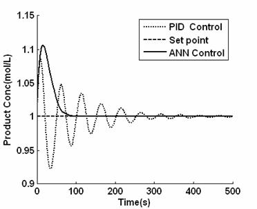
Figure 9. Closed loop responses of the in the presence of disturbance
In order study system robustness we introduce plant-model mismatch where a 20% change in the parameter (ΔH/ρCp) was applied to the.
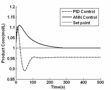
Figure 10. Closed loop responses of the system in the presence of uncertainty
Figure 10: shows the response, it is seen that ANN controller returned the system to its origin after 300s controller which shows that the response was very slow; the system did not settled on time. There was also overshoot of around 10%. For the case of PID controller, the response was fast and there was overshoot and inverses response. The controller could not eliminate steady state error. The ANN controller performed much slower than PID control scheme during both plant model mismatch and disturbances rejection simulation.
Conclusions
From the results obtained in our simulation we can see that the ANN controller using model reference was able to track set point change and reject the uncertainties resulting from external disturbances and plant model mismatches. The responses were somehow sluggish in the faces of external disturbances but give no oscillatory behaviors. For PID controller, the performance deteriorated for set point changes and under the influence of external disturbances. This reason for poor performance can be adduced because of high nonlinearity of the CSTR.
ANN control approach using references model to tailor system output to a desired responses was developed. The controller has been able to take care of nonlinearly aspect of the system. ANN control scheme has better trajectory tracking ability than PID since the former is based on nonlinearity of the model, while the latter based on particular operating conditions. The control was able to adapt to system changes and operating condition change. There was no need for turning parameter in the control. The control was very adaptive and has self-turning capability for any change in operating conditions and system parameters. During the online implementation, the networks ware continuously adapted online, the controller did not require an integral action to obtain zero offset in the system output. The proposed method is somehow sluggish because the optimal control action is iterative in order to converge to an acceptable accuracy.
Reference
[1] Findeison R., Island L., F. Allgower, Foss B. A., Output feedback Stabilization for constrained systems with non-linear model predictive control, Int.J. of robust and non-linear control 13(3- 4), 2003, p. 211-227.
[2] Cybenko G., Approximation by super position of a sigmoidal function, Mathematics of control, signals and system, Vol.2, No.4, 1989, p. 303-314.
[3] Neural Network Toolbox User Guide, October, 1998, the math works Inc.
[4] Saerens M., Soquet A., Neural Controller based on back propagation algorithm, IEE proceeding F, vol. 138, no. 1, 1991, p. 55-62.
[5] Chlamreza Zahedi Abdolhessin Jahanmiri, Rahimpor M. R., Neural network approach for prediction of the CUO-ZnO-AL2O3 catalyst deactivation, Int-J. of chemical Reactor engineering, Vol .3, 2005, A8.
[6] Barto, Sutton, Anderson, Neuron like adaptive elements that can solve difficult leaning control problem, IEE Transon systems, man and cybernetics, Sept - Oct 1983, VOL SMC-13, 1983, pp. 834-846.
[7] Hunt and Sberbaro, Neural Networks for control system - A survey, Automatic, vol.28, 1992, p. 1083-1112.
[8] Aris R., Amunson N. R., An analysis of chemical reactor stability and control - I,II, Chem. Ey.Sci, 7, 1958, p. 121-147.
[9] Hagan M., Demuth H., Neural network Design, Boston, PWS, 1996.
[10] Mohd Hussain, Pei Vee Ho, Adaptive sliding mode control with neural network based hybrid models, J. of Process Control, 14, 2004, p. 1578-1576.
[11] Blenoxx G. A., Montaque, Frith A. M., Chris G., Bevan V., Industrial Application of neural networks - on investigation, J. process control, 11, 2001, p. 497-507.
[12] Levenberg K., A method for the solution of certain non-linear problems least squares, Quart. Appl. Math., 2, 1944, p. 164-168.
[13] Marquardt D. W., An algorithim for least-square astimation of non linear parameters, J.soc. Ind. Appl. Math., 11, 1963, p. 431-441.
[14] M.L thompson, M.K kramer, Modelling Chemical Process using prior Knowledge and Neural networks, AICHEJ. 40(1994.) 1340.
[15] Atom K. J., Hagglund T., P/D controller: theory design and turning, Instrument society of America, 1995.
[16] Psichogious D. C., Ungar L. H., Direct and indirect model based control artificial neural networks, Ind. Eng. Chem. Res., 30, 1991, p. 2564.
[17] Nahas E. P., Henson M. A., Serborg D. E., Nonlinear internal model control strategy for neural network models, Comput. Chem Eng., 16, 1992, p. 1039.
[18] Nikolaou M., Hanagendu V., Control of nonlinear dynamic systems modeled by recurrent neural network, A. M. Inst. Chem. Eng. J., 39, 1993, p. 1890
[19] Fuli N., Mingzhong L., Yinghua Y., Neural network pole placement controller for nonlinear systems through linearization, American control conference 1997, p.1984.