Markov Decision Model and the Application to the Cost of Treatment of Leprosy Disease

 

Usman Yusuf ABUBAKAR¹, Sunday A. REJU² and Bamidele O. AWOJOYOGBE³

 

¹Department of Mathematics and Computer Science, Federal University of Technology, Minna, Nigeria

²National Open University, Lagos, Nigeria

³Department of Physics, Federal University of Technology, Minna, Nigeria

abbkruy@yahoo.com

 

 

Abstract

A Markov decision model is applied to determine the optimal cost of drugs in the treatment of leprosy disease. The result shows that the minimum cost is obtained if the Doctor is visited and the patient is placed on the MDT instead of traditional treatment and Dopsone monotherapy. The paper presents a theoretical framework to study the cost of treatment of leprosy where the relevant data could be obtained.

Keywords

Markov Chain, Decision; Leprosy; Treatment; Cost; Dopsone - Monotherapy; Multi-Drug Therapy

 

 

Introduction

 

Leprosy is an infectious disease of the skin and nerves caused by mycobacterium Leprae. It is wide spread in the tropical and sub tropical countries including Nigeria. Leprosy can be treated and cured with the Multi-Drug Therapy (MDT) or Dapsone-Monotherapy even without the associated deformity if it was detected early [1],[2]. Prevalence rate and incidence of new cases of leprosy has be studied [3]. In addition, kinship coefficient has been used to study leprosy rates in villages of different distance apart [4]. In a related study, [5] has studied the relapses in leprosy after treatment with Dapsone-monotherapy and Multi-Drug-Therapy (MDT) respectively. In this paper, we determine the best alternative in terms of drug-type in the treatment of leprosy disease.

 

 

The Model Equations

Let X_n denote the state of the process at time n and a_n the action chosen at time n, then the above is equivalent to stating that:

P(Xn+1=j|X0,a0, X1,a1,…..Xn=i, an=a)  = Pij(a)

(1)

 

This is the transition probability of a visit to state j given that state i was last visited when action a was chosen. Thus the transition probabilities are dependent on the present state and subsequent action [6].

A policy; by a policy we mean a rule for choosing actions. A policy is a sequence of decisions, one for each state of the process. It is denoted by d_i⁽ⁿ⁾ where n = 1, 2, …  represent time  and i = 1, 2,….represent state.

Following [[7]], we consider an aperiodic, irreducible Markov chain with m states (m<) and the transition probability matrix:

 

With every transition i to j associate a reward R_ij. If we let V_i⁽ⁿ⁾ be the expected total earnings (reward) in the next n transitions, given that the system is in state i at present . A simple recurrence relation can be given for  as follows:

where i = 1,2,3,…..,m; n  =  1,2 …

(2)

 

Let

Equation (2) can now be written as

(3)

setting n= 1,2,…. we get

where P_ij⁽ⁿ⁾ is the (i,j)^th element of the matrix Pⁿ

Let

Equation (3) can be put in matrix notation as

Extending this to a general n, we have

 

Theorem 1

Let  be the n-step transition probability of an aperiodic, irreducible, m-tate Markov chain. Let  be the limiting probabilities. Then there exist constants c and r with c > 0 and 0 < r < 1, such that  where

Proof

From [7], we know that

and hence

From [7], we also have ; setting n = kN + 1, we get k = (n - 1)/N and

 

The theorem now follows by setting c = (1-2ε_n)^-1 and r = (1-2ε_n)^1/n.

Consequently,

Where is the limiting distribution of the Markov chain and with c > 0 and 0 < r < 1. Therefore, as ,  geometrically.

            Let  and

In Matrix notation, we can write P^­­n as

Substituting this in (3) we get:

(4)

In deriving (4), we have noted that  

Now consider the sum

(5)

 

It should be noted that each term in is less than or equal to cr^k (c > 0,0 < r < 1) in absolute value, and hence for large n the second term on the right hand side of (5) approaches an m x m matrix with zero elements. For the same reason the last term in (4) approaches a null matrix for large n.

Thus, asymptotically we have

 

which gives

(6)

where we have written

writing

and

 

so that (6) can be put in the form

which shows that for large n, is a linear function of q for every i. Further, for different values of i,are represented by parallel straight lines with slope q and intercept

So far, we have considered the transition probability matrix P and the reward matrix R as given.

Instead, suppose that the decision maker has other alternatives and so is able to alter elements of P and R. To incorporate this feature, we define D as the decision set, and under decision KD, let ^KP_ij and ^KR_ij be the probability of the transition from i to j and the corresponding reward respectively for ^Kv_i^(n). The expected total earnings in n transitions under decision K; we have the recurrence relations (K=0 represents the optimal decision)

(7)

giving

where we have written

Recursive relation (7) gives an iteration procedure to determine the optimum decision d_i⁽ⁿ⁾D. For i=1,2…m and n=1,2…

This is a Standard technique in Dynamic programming and it has been shown by Bellman [8],[9], that this iteration process will converge on best alternative for each state as.

The method is based on recursively determining the optimum policy for every n, that would give the maximum value.

However, one major drawback of the method is that, there is no way to say when the policy converges into a stable policy; therefore, the value iteration procedure is useful only when n, is fairly small

 

 

Application

 

We consider a new case of leprosy, that is, a person showing clinical signs of leprosy, with or without bacteriological confirmation of the diagnosis (state 1), or a new case with WHO disability grade 1 (state 2), or a new case with WHO disability grade 2 (state 3) [1,2]. Thus, we have a three states model. We assumed that all the states communicate (Ergodic). Let the transition between the states be represented by the transition diagram shown in figure 1, governed by the following transition probabilities of Markov chain in (1) and Markov reward matrices respectively.

 

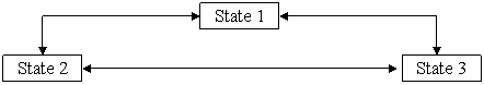
Figure 1. The Transition Diagram for Leprosy Patients

 

….where 0 £ p_ij £ 1 and , i = 1,2 and 3 and ; i, j = 1, 2, 3.

Figure 2 presented the possible realization of the state transitions.

 

Figure 2. A possible realization of the state transitions

 

At any given point in time and state of the disease; the patient has the opportunity or a privilege to make a choice of drugs. The choice of drugs may however be dependent on the availability of the drugs, resources available to the patient and the state or severity of the disease. The two major types of drugs used for the treatment of leprosy are Dapsone- Monotherapy and Multi-Drug therapy (MDT) [1,2] respectively.

For the sake of simplicity we may further divide the drugs into Low priced drugs and high priced drugs to correspond to Dapsone and MDT respectively. We shall have the following alternatives for the states [10]:

·        State1:

o       Alternative 1: Self-medication (Traditional treatment)

o       Alternative 2: Go to see a doctor (cost of seeing a Doctor).

·        State 2:

o       Alternative 1: Low priced drugs

o       Alternative 2: high price drugs

·        State 3:

o       Alternative 1: Continue without change of drugs

o       Alternative 2: Change drugs (from low to high priced or vice versa).

Costs are associated with each of these alternatives.

Our objective is to obtain the policy or alternative that minimizes the costs of the treatment at any given state and time.

Let the transition probabilities (P_ij) and the corresponding reward (R_ij) be given as follows:

; i, j = 1 ,2, 3

and

; i, j = 1 ,2, 3

Let D be the decision set and we have two Alternative decisions available to the patient. That is, Alternative 1; and Alternative 2; Thus in every state we have k=1,2D.

We shall now determine the best policies for every n using equation (7).

Since we are concerned about minimizing the costs of drugs to be administered; the alternative that yields the least value constitutes the best policy for the state and time.

 

 

Results

 

Suppose we have the following stationary transition probabilities and the corresponding cost matrices.

and

in N 1000 respectively

The subsequent transition probabilities and cost matrices are given below when the decisions are implemented.

            and      

i, j = 1, 2, 3 for k = 1                            i, j = 1, 2, 3 for k =1

            and      

i, j = 1, 2, 3 for k = 2                            i, j = 1, 2, 3 for k = 2

We shall use these values to determine the best polices for each n.

The summary of the results is presented in Table1.

 

Table 1. A Summary result of the Optimal Policies and Costs

 

 

Discussion

 

The results indicate the best policies for each n. d_i⁽ⁿ⁾ where n = 1, 2, 3,4, 5 and i = 1, 2, 3.Thus, we have obtained the best policies for the three states for five years. In addition to the best policies, the corresponding expected minimum costs are also provided. For instance, d₁⁽¹⁾ = 2 with ^oV₁⁽¹⁾ = 1,200 means that the best policy for state 1 for the first year is to see the doctor and the corresponding expected minimum cost is one thousand and two hundred Naira (N 1200.00).

The results revealed that except for the d₂ ⁽¹⁾ = 1 with the corresponding ^oV₂⁽¹⁾ = 2,300, the best policy for the other states at each time is the alternative 2. Which means that the best policy for each other state at each time is the second alternative. This is a kind of convergence to a stable policy The convergence is so smooth that further iteration beyond five years is not necessary. This type of convergence is not generally true of this iterative algorithm, however, it makes this illustration very interesting.

 

 

References