A Simplified Dynamic Model for Constant-Force Compression Spring
Ikechukwu Celestine UGWUOKE
Department of Mechanical Engineering, Federal University of Technology, Minna, Niger State, Nigeria.
E-mail(s):ugwuokeikechukwu@yahoo.com
Abstract
A simplified dynamic model for the constant-force
compression spring (CFCS) based on the pseudo-rigid-body model (PRBM) is
presented including the basic formulations which takes care of the moment ![]() due to
coulomb friction in the pin joints of the CFCS, and the moment
due to
coulomb friction in the pin joints of the CFCS, and the moment ![]() due to
axial force effects in the rigid links of the CFCS. The CFCS is a slider
mechanism which consists of rigid links incorporating pin joints and a small-length
flexural pivot which connects to a slider. Clearly the results with the
inclusion of
due to
axial force effects in the rigid links of the CFCS. The CFCS is a slider
mechanism which consists of rigid links incorporating pin joints and a small-length
flexural pivot which connects to a slider. Clearly the results with the
inclusion of ![]() and
and ![]() to the dynamic model, shows
that the static terms
to the dynamic model, shows
that the static terms ![]() have very great significance on the dynamic
model of the CFCS.
have very great significance on the dynamic
model of the CFCS.
Keyword
Constant-force compression spring, Axial force effects, Coulomb friction, Pseudo-rigid-body model.
Introduction
With the emerging applications of compliant mechanisms, there is the need to develop a systematic formulation for the design and analysis of compliant mechanisms. Although existing methods such as the finite element method (FEM), elliptic integrals method, and chain algorithm method are widely available, there remain challenges in the computational model of compliant mechanisms (CMs). Many of these existing models are either inadequate to capture the geometric nonlinearity or too complicated that they cannot serve as a basis for compliant mechanism (CM) design and simulation. Based on the principle of dynamic equivalence, a simplified dynamic model for the constant-force compression spring (CFCS) is developed using the pseudo-rigid-body (PRB) modeling technique. The pseudo-rigid-body model (PRBM) is used to simplify the analysis and design of CMs. It is used to unify CM and rigid-body mechanism theory by providing a method of modeling the nonlinear deflection of flexible beams. This method of modeling allows well-known rigid-body analysis methods to be used in the analysis of CMs (Salamon, 1989). The PRBM provides an easy way to model the complex, nonlinear deflections of many CMs (Howell, 2001). The model approximates the force-deflection characteristics of a compliant segment using two or more rigid segments joined by pin joints, with torsional springs at the joints modeling the segment’s stiffness. The usefulness of the PRBM in allowing accurate analysis and synthesis of mechanism motion and energy storage characteristics has been abundantly demonstrated (Opdahl et al., 1998; Derderian et al., 1996; Howell and Midha, 1996; Lyon et al., 1997; Jensen et al., 1997; Mattlach and Midha, 1996). While the model is very useful for the analysis of CMs, its true power lies in the capability it gives for designing original CMs (Jensen et al.’ 1997). The PRBM correlates the synthesis of CMs and the wealth of knowledge available in rigid-body mechanism design. CFCSs can be defined as mechanisms that produce a constant output force for a large range of input displacements. Such mechanisms are important in applications with varying displacements, but requiring a constant resultant output force. The mechanism is typically displacement driven, the input is a displacement at the slider and the output is a force. Unlike a linear spring where the force increases as the displacement increases, the reaction force for a CFCS remains constant for various displacements.
Simplified Dynamic Model Development
Figure 1 shows the CFCS and its PRBM. As shown in the figure, the CFCS consists of rigid links incorporating pin joints and a small-length flexural pivot which connects to a slider. The mechanism is converted to its rigid-body counterpart by using the PRBM rule for small-length flexural pivots. The most straight forward alteration is that the small-length flexural pivot becomes a pin and torsional spring combination, centered at the middle of the flexible segment. The torsional spring constant K for small-length flexural pivots is given by
K=EI/L (1)
Where,
I is the moment of inertia of the cross section of the flexible segment
E is the modulus of elasticity of the flexible segment
L is the length of the flexible segment
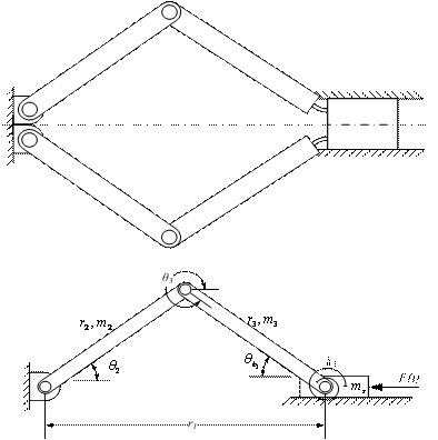
Figure 1: CFCS and Its pseudo-rigid-body model
Formulation of the Dynamic Equation using Hamilton’s Principle
The dynamic equation of motion for the CFCS can be systematically derived using Hamilton’s principle, where the following variational form holds:
![]() (2)
(2)
Equation (2), which is generally known as Hamilton’s
variational statement of dynamics, shows that the sum of the time-variations of
the difference in kinetic and potential energies and the work done by the
nonconservative forces over any time interval ![]() equals zero. It is of
interest to note that Hamilton’s
equation can also be applied to statics problems. In this case, the kinetic
energy term
equals zero. It is of
interest to note that Hamilton’s
equation can also be applied to statics problems. In this case, the kinetic
energy term ![]() vanishes, and the remaining terms in
the integrands of equation (2) are invariant with time; thus, equation (2)
reduces to
vanishes, and the remaining terms in
the integrands of equation (2) are invariant with time; thus, equation (2)
reduces to
![]() (3)
(3)
Equation (3) is the well known principle of minimum potential energy, so widely used in static analysis. For most mechanical or structural systems, the kinetic energy can be expressed in terms of the generalized coordinates and their first time derivatives, and the potential energy can be expressed in terms of the generalized coordinates alone (Clough and Penzien, 2003). In addition, the virtual work which is performed by the nonconservative forces as they act through the virtual displacements caused by an arbitrary set of variations in the generalized coordinates can be expressed as a linear function of those variations. In mathematical terms the above three statements are expressed in the form
![]() (4)
(4)
![]() (5)
(5)
![]() (6)
(6)
where the coefficients ![]() are the generalized forcing functions
corresponding to the coordinates
are the generalized forcing functions
corresponding to the coordinates ![]() respectively. Substituting equation (4),
(5), and (6) into (2) and completing the variation of the first term gives
respectively. Substituting equation (4),
(5), and (6) into (2) and completing the variation of the first term gives
 (7)
(7)
Integrating the velocity-dependent terms in equation (7) by paths leads to
 (8)
(8)
The first term on the right hand side of equation (8) is
equal to zero for each coordinate since ![]() is the basic condition imposed upon the
variations. Substituting equation (8) into equation (7) gives, after
rearranging terms,
is the basic condition imposed upon the
variations. Substituting equation (8) into equation (7) gives, after
rearranging terms,
 (9)
(9)
where ![]() are the kinetic and potential energy of
the CFCS respectively. Since all variations
are the kinetic and potential energy of
the CFCS respectively. Since all variations ![]() are arbitrary, equation (9)
can be satisfied in general only when the term in bracket vanishes.
are arbitrary, equation (9)
can be satisfied in general only when the term in bracket vanishes.
 (10)
(10)
Equations (10) are the well known Lagrange’s equations of motion, which have found widespread application in various fields of science and engineering. It should be noted that Lagrange’s equations are a direct result of applying Hamilton’s variational principle, under the specific condition that the energy and work terms can be expressed in terms of the generalized coordinates, and of their time derivatives and variations. Thus Lagrange’s equations are applicable to all systems which satisfy these restrictions, and they may be nonlinear as well as linear (Clough and Penzien, 1995). Following the standard procedure of Hamilton’s principle, the total kinetic energy equation for the CFCS is given as
![]() (11)
(11)
where,
![]() = mass of links 2 and 3
= mass of links 2 and 3
![]() = velocity of the center of mass of
links 2 and 3
= velocity of the center of mass of
links 2 and 3
![]() = mass moment of inertia of links 2 and
3 about the center of mass
= mass moment of inertia of links 2 and
3 about the center of mass
![]() = angular velocity of links 2 and 3
= angular velocity of links 2 and 3
![]() = velocity of the slider
= velocity of the slider
![]() (12)
(12)
 (13)
(13)
![]() (14)
(14)
 (15)
(15)
The first three terms of the kinetic energy expression represent the translational energy of the system, and the last two represent the rotational energy. The mass moments of inertia of links 2 and 3 about the center of mass is given by
![]() (16)
(16)
For the CFCS, the potential energy equation is given as
![]() (17)
(17)
where ![]() is the torsional spring constant and
is the torsional spring constant and ![]() is the
relative deflections of the torsional spring given by the following expression
is the
relative deflections of the torsional spring given by the following expression
 (18)
(18)
Expanding equation (10) and simplifying, the dynamic equation for the system becomes

(19)
To obtain the generalized forcing function ![]() , the
virtual work
, the
virtual work ![]() must be evaluated. This is the work
performed by all nonconservative forces acting on or within the flexural member
while an arbitrary set of virtual displacements is applied to the system. The
nonconservative forces may include dissipative forces proportional to the
angular and linear velocities. For the CFCS, the generalized forcing function
must be evaluated. This is the work
performed by all nonconservative forces acting on or within the flexural member
while an arbitrary set of virtual displacements is applied to the system. The
nonconservative forces may include dissipative forces proportional to the
angular and linear velocities. For the CFCS, the generalized forcing function ![]() therefore
consists of a moment
therefore
consists of a moment ![]() due directly to the force
due directly to the force ![]() acting
on the slider, moment
acting
on the slider, moment ![]() due to coulomb friction in the pin
joints of the CFCS, and moment
due to coulomb friction in the pin
joints of the CFCS, and moment ![]() due to axial force effects in the rigid
links of the CFCS. In mathematical terms, the generalized forcing function
due to axial force effects in the rigid
links of the CFCS. In mathematical terms, the generalized forcing function ![]() is given by
the expression below
is given by
the expression below
![]() (20)
(20)
Coulomb friction results from two dry or lubricated
surfaces rubbing together. It is generally considered to be independent of
velocity magnitude but has a different, larger value when velocity is zero
(static friction) than when there is relative motion between the parts (dynamic
friction). Though more elaborate expressions for the coulomb friction term ![]() are
possible, the following simple relation gives sound results:
are
possible, the following simple relation gives sound results:
 (21)
(21)
where C is the coulomb friction coefficient
 (22)
(22)
The value of the torque ![]() is chosen using experimental
data but may be approximated using the expression giving in equation (22).
Torque
is chosen using experimental
data but may be approximated using the expression giving in equation (22).
Torque ![]() is
transformed to mechanism’s output force F using the power relationship given
as:
is
transformed to mechanism’s output force F using the power relationship given
as:
![]() (23)
(23)
 (24)
(24)
where,
 (25)
(25)
Equations (19)–(25) represent the simplified dynamic model of the CFCS. Note that the equation of motion was derived from the PRBM of the CFCS, rather than the actual CFCS. What is important in the derivation of the dynamic model is not the method chosen to arrive at the simplified dynamic model, but the fact that the method was applied to the PRBM simplification of the CFCS.
Results and Discussion
All the necessary parameters of the CFCS used in the
simulation are given in table 1. Using these parameters, the simulation results
obtained are illustrated in the following figures. Figure 2 shows a comparison
of the force predicted by the static portion of the dynamic model (i.e. with
velocities and accelerations set to zero, with![]() ), with that predicted by
existing CFCS theory, essentially an application of the principle of virtual
work on the PRBM of the CFCS. As shown in the figure, both plots match
perfectly which is a confirmation that the static portion of the dynamic model
is correct. Figure 3 shows the force predicted by the static portion of
the dynamic model with inclusion of
), with that predicted by
existing CFCS theory, essentially an application of the principle of virtual
work on the PRBM of the CFCS. As shown in the figure, both plots match
perfectly which is a confirmation that the static portion of the dynamic model
is correct. Figure 3 shows the force predicted by the static portion of
the dynamic model with inclusion of![]() . As shown in the figure,
. As shown in the figure, ![]() have large
effect on the performance of the CFCS.
have large
effect on the performance of the CFCS.
Table 1: CFCS parameters used for simulation
|
Parameters |
Parameter Values |
|
r2 |
85 mm |
|
r3 |
95 mm |
|
m2 |
0.025kg |
|
m3 |
0.028 kg |
|
ms |
0.087kg |
|
b |
25.4 mm |
|
|
0.38 mm |
|
|
1.1615 x 10⁻¹³ m4 |
|
E |
207 Gpa |
|
|
9.5 mm |
|
|
2.5308 Nm |
|
|
0.045 rad |
|
|
0.02 |
Figure 5, 6, and 7 shows the mean force plot, the median
force plot and the peak-to-peak force magnitude difference plot of the dynamic
model as a function of frequency respectively. Each frequency assumes a
sinusoidal position input as shown in Figure 4 with amplitude equal to 40%
mechanism deflection. Notice that the curve in the peak-to-peak force plots for
the dynamic model with the inclusion of ![]() and
and ![]() first curves down, before it
starts to increase. This shows the range of frequencies over which a CFCS
exhibits better constant force behaviour. Figure 8, 9, 10, and 11 shows the
plots of the force predicted by the dynamic model with, and without the
inclusion of the static terms
first curves down, before it
starts to increase. This shows the range of frequencies over which a CFCS
exhibits better constant force behaviour. Figure 8, 9, 10, and 11 shows the
plots of the force predicted by the dynamic model with, and without the
inclusion of the static terms ![]() for different input frequencies.
Clearly as shown in the figures, the results with the inclusion of
for different input frequencies.
Clearly as shown in the figures, the results with the inclusion of![]() , shows that
the static terms
, shows that
the static terms ![]() have very great significance on the
dynamic model. Figure 12 shows the plot of the percent constant-force (PCF) as
a function of time. The PCF is very important because it measures the amount of
variation between the minimum and maximum output force of the CFCS model. As
shown in the figure, the maximum value of the PCF for the CFCS model is 87.2%.
have very great significance on the
dynamic model. Figure 12 shows the plot of the percent constant-force (PCF) as
a function of time. The PCF is very important because it measures the amount of
variation between the minimum and maximum output force of the CFCS model. As
shown in the figure, the maximum value of the PCF for the CFCS model is 87.2%.
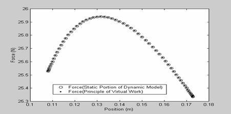
Figure 2: Force predicted by the static portion of the dynamic model
with that predicted by the principle of virtual work
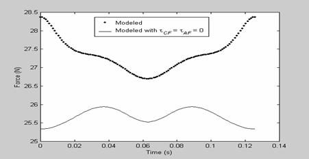
Figure 3: Force predicted by the static portion of the dynamic model
with inclusion of tCF and tAF
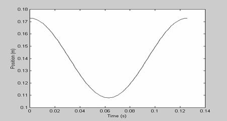
Figure 4: Position plot representing the sinusoidal input
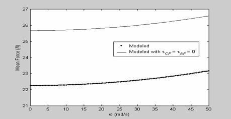
Figure 5: The mean force plot as a function of frequency for the CFCS
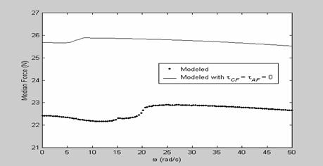
Figure 6: The median force plot as a function of frequency for the CFCS
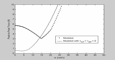
Figure 7: The peak-to-peak force difference plot as a function of frequency for the CFCS
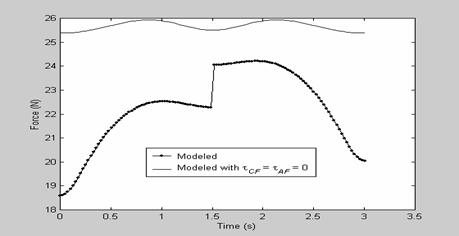
Figure 8: Predicted force for sinusoidal input of ω = 2.09 rad/s
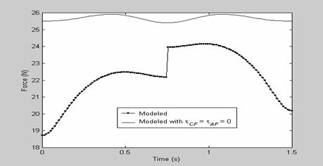
Figure 9: Predicted force for sinusoidal input of ω = 4.19 rad/s
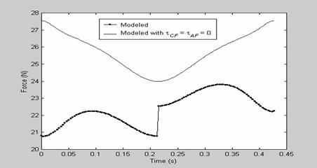
Figure 10: Predicted force for sinusoidal input of ω = 14.7 rad/s
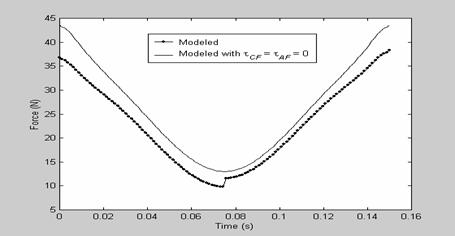
Figure 11: Predicted force for sinusoidal input of ω = 41.89 rad/s
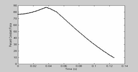
Figure 12: Percent constant-force as a function of time
Conclusion
The PRBM is a method of analysis that allows large
deformations to be modeled using rigid-body kinematics. In light of the
simplicity the PRBM affords, a simplified dynamic model for the CFCS based on
the PRBM is presented which also includes basic formulations which take care of
the axial force effects in the rigid links of the CFCS and the effect due to
Coulomb friction in the pin joints of the CFCS. Although several methods for
modeling CFCS exist, less attention has been paid to dynamic analysis. A very
interesting aspect of the dynamic model is that it presents a very simplified
and accurate mathematical expression which helps in the easy determination of
the moment ![]() due to coulomb friction in the pin
joint of the CFCS, and the moment
due to coulomb friction in the pin
joint of the CFCS, and the moment ![]() due to axial force effects in the rigid
links of the CFCS. Clearly the results with the inclusion of
due to axial force effects in the rigid
links of the CFCS. Clearly the results with the inclusion of ![]() and
and ![]() to the
dynamic model, shows that the static terms
to the
dynamic model, shows that the static terms ![]() have very great significance
on the dynamic model of the CFCS.
have very great significance
on the dynamic model of the CFCS.
References
1. Derderian, J. M., “The Pseudo-Rigid-Body Model Concept and its Application to Micro Compliant Mechanisms”, M. S. Thesis, Brigham Young University, Provo, Utah. 1996.
2. Jensen, B. D., Howell, L. L., Gunyan, D. B., and Salmon, L. G., “The Design and Analysis of Compliant MEMS Using the Pseudo-Rigid-Body Model”, Microelectromechanical Systems (MEMS) 1997, 1997 ASME International Mechanical Engineering Congress and Exposition, Nov. 16-21, 1997, Dallas, TX, DSC-Vol. 62, pp. 119-126, 1997.
3. Lyon, S. M., Evans, M. S., Erickson, P. A., and Howell, L. L, “Dynamic Response of Compliant Mechanisms Using the Pseudo-Rigid-Body Model”, Proceedings of the 1997 ASME Design Engineering Technical Conferences, DETC97/VIB-4177, 1997.
4. Howell, L. L., and Midha, A., ‘‘A Loop-Closure Theory for the Analysis and Synthesis of Compliant Mechanisms,’’ ASME Journal of Mechanical Design, 118, No. 1, pp. 121–125, 1996.
5. Howell, L. L., “Compliant Mechanisms”, John Wiley & Sons, New York, 2001.
6. Opdahl, P. G., Jensen, B. D., and Howell, L. L., “An Investigation into Compliant Bistable Mechanisms”, Proc. of 1998 ASME Design Engineering Technical Conferences, DETC98/MECH-5914, 1998.
7. Mettlach, G. A., and Midha, A., “Using Burmester Theory in the Design of Compliant Mechanisms”, Proceedings of the 1996 ASME Design Engineering Technical Conferences, 96-DETC/MECH-1181, 1996.
8. Salamon, B. A., “Mechanical Advantage Aspects in Compliant Mechanisms Design”, M.S. Thesis, Purdue University, West Lafayette, Indiana, 1989.
9. Clough, R.W.; and Penzien, J., “Dynamics of Structures”, Third Edition, Computer and Structures, Inc., University Ave. Berkeley, CA 94704, USA, 2003.