Ant Colony Optimization Applied on Combinatorial Problem for Optimal Power Flow Solution

Brahim GASBAOUI and Boumediène ALLAOUA^*

Bechar University, Faculty of Sciences and Technology, Department of Electrical Engineering,

B.P 417 BECHAR (08000) Algeria

E-mail(s): gasbaoui_2009@yahoo.com, elec_allaoua2bf@yahoo.fr

(*Corresponding Author)

Abstract

This paper presents an efficient and reliable evolutionary-based approach to solve the optimal power flow (OPF) combinatorial problem. The proposed approach employs Ant Colony Optimization (ACO) algorithm for optimal settings of OPF combinatorial problem control variables. Incorporation of ACO as a derivative-free optimization technique in solving OPF problem significantly relieves the assumptions imposed on the optimized objective functions. The proposed approach has been examined and tested on the standard IEEE 57-bus test System with different objectives that reflect fuel cost minimization, voltage profile improvement, and voltage stability enhancement. The proposed approach results have been compared to those that reported in the literature recently. The results are promising and show the effectiveness and robustness of the proposed approach.

Keywords

Optimal Power Flow; Ant Colony Optimization; Combinatorial Optimization; Power Systems; Metaheuristic.

Introduction

In the past two decades, the problem of optimal power flow (OPF) has received much attention. It is of current interest of many utilities and it has been marked as one of the most operational needs. The OPF problem solution aims to optimize a selected objective function such as fuel cost via optimal adjustment of the power System control variables, while at the same time satisfying various equality and inequality constraints. The equality constraints are the power flow equations, while the inequality constraints are the limits on control variables and the operating limits of power system dependent variables. The problem control variables include the generator real powers, the generator bus voltages, the transformer tap settings, and the reactive power of switchable VAR sources, while the problem dependent variables include the load bus voltages, the generator reactive powers, and the line flows. Generally, the OPF problem is a large-scale highly constrained nonlinear optimization problem.

Useful OPF is limited by the high dimensionality of power systems and the incomplete domain dependent knowledge of power system engineers. The first limitation is addressed by numerical optimization procedures based on successive linearization using the first and the second derivatives of objective functions and their constraints as the search directions or by linear programming solutions to imprecise models [1, 2]. The advantages of such methods are in their mathematical underpinnings, but disadvantages exist also in the sensitivity to problem formulation, algorithm selection and usually converge to local minima [3]. The second limitation, incomplete domain knowledge, precludes also the reliable use of expert systems where rule completeness is not possible. In the evolutionary and adaptive algorithms one of the most recent is the Ant Colony Optimization (ACO) computational paradigm introduced by Marco Dorigo in his Ph.D. thesis in 1992 [4], and expanded it in his further work, as summarized in [5, 6, 7].

A new powerful approach of ACO is accessible to these optimization problems made possible by the increasing availability of high performance computers at relatively low costs. As the name suggests, these algorithms have been inspired in the real ant colonies behavior. When searching for food, ants initially explore the area surrounding their nest in a random manner. As soon as an ant finds a food source, it evaluates quantity and quality of the food and carries some of the found food to the nest. During the return trip, the ant deposits a chemical pheromone trail on the ground. The quantity of pheromone deposited, which may depend on the quantity and quality of the food, will guide other ants to the food source. The indirect communication between the ants via the pheromone trails allows them to find shortest paths between their nest and food sources. This functionality of real ant colonies is exploited in artificial ant colonies in order to solve global optimization searching problems when the closed-form optimization technique cannot be applied.

Characters of the ACO algorithms use the parameters, probabilistic model that is used to generate solutions to the problem under consideration. The probabilistic model is called the pheromone model. The pheromone model consists of a set of model parameters, which are called the pheromone trail parameters. The pheromone trail parameters have values, called pheromone values. At run-time, ACO algorithms try to update the pheromone values in such a way that the probability to generate high-quality solutions increases over time. The pheromone values are updated using previously generated solutions. The update aims to concentrate the search in regions of the search space containing high-quality solutions. In particular, the reinforcement of solution components depending on the solution quality is an important ingredient of ACO algorithms. It implicitly assumes that good solutions consist of good solution components. To learn which components contribute to good solutions can help to assemble them into better solutions.

ACO methods have been successfully applied to diverse combinatorial optimization problems including travelling salesman [8, 9], quadratic assignment [10, 11], vehicle routing [12, 13, 14], telecommunication networks [15], graph colouring [16], constraint satisfaction [17], Hamiltonian graphs [18], and scheduling [19, 20, 21].

This paper presents the application of the ant colony optimization algorithms in the Optimal Power Flow (OPF) combinatorial problem applied on IEEE 57-bus Electrical Network. The algorithm was developed MATLAB environment programming (R2008a, v7.6).

Problem Formulation

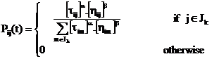
Optimal Power Flow is defined as the process of allocating generation levels to the thermal generating units in service within the power system, so that the system load is supplied entirely and most economically [30, 31]. The objective of the OPF problem is to calculate, for a single period of time, the output power of every generating unit so that all demands are satisfied at minimum cost, while satisfying different technical constraints of the network and the generators. The problem can be modeled by a system which consists of ng generating units connected to a single bus-bar serving an electrical load Pd. The input to each unit shown as F_i, represents the generation cost of the unit. The output of each unit Pg_i is the electrical power generated by that particular unit. The total cost of the system is the sum of the costs of each of the individual units.

The essential constraint on the operation is that the sum of the output powers must equal the load demand. The standard OPF problem can be written in the following form:

(1)

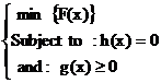
where F(x) the objective function, h(x) represents the equality constraints, g(x) represents the inequality constraints and x is the vector of the control variables, that is those which can be varied by a control center operator (generated active and reactive powers, generation bus voltage magnitudes, transformers).

Objective Function

Generally, the OPF problem can be expressed as minimizing the cost of production of the real power which is given by objective function F_T

where,

(2)

The fuel cost function or input-output characteristic of the generator may be obtained from design calculations or from heat rate tests. Many different formats are used to represent this characteristic. The data obtained from heat rate tests or from the plant design engineers may be fitted by a polynomial curve. It is usual that, quadratic characteristic is fit to these data. A series of straight-line segments may also be used to represent the input-output characteristic [30]. The fuel cost function of a generator that usually used in power system operation and control problem is represented with a second-order polynomial.

(3)

Where ng is the number of generation including the slack bus. Pg is the generated active power at bus i. a_i - b_i  and c_i are the unit costs curve for i^th generator.

The standard OPF problem can be described mathematically as an objective with two constraints as:

	(4)
	(5)

where:

: Real power output of i-th generator (MW);

F_T: Total Operating cost ($ /h);

: Operating cost of unit i ($ /h);

Pd: Total demand (MW);

P_L: Transmission losses (MW);

: Operating power limits of unit i (MW);

ng: Total number of units in service.

Optimal Power Flow Using Ant Colony Optimization

Ant colony optimization method description

In the ant colony optimization (ACO), a colony of artificial ants cooperates in finding good solutions to difficult optimization problems. Cooperation is a key design component of ACO algorithms: The choice is to allocate the computational resources to a set of relatively simple agents (artificial ants) that communicate indirectly by stigmergy. Good solutions are an emergent property of the agent’s cooperative interaction.

Artificial ants have a double nature. On the one hand, they are an abstraction of those behavioral traits of real ants which seemed to be at the heart of the shortest path finding behavior observed in real ant colonies. On the other hand, they have been enriched with some capabilities which do not find a natural counterpart. In fact, we want ant colony optimization to be an engineering approach to the design and implementation of software Systems for the solution of difficult optimization problems. It is therefore reasonable to give artificial ants some capabilities that, although not corresponding to any capacity of their real ant’s counterparts, make them more effective and efficient.

Each ant generates a complete tour by choosing the cities according to a probabilistic state rule. Mathematically, the probability with which ant k in city r chooses to move to the city s is [22]:

(6)

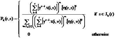
where τ is the pheromone, η is the visibility which is the inverse of the distance δ(r,s), J_k(r) is the set of cities that remain to be visited by ant k positioned on city r , α and β are two coefficients which make the pheromone information or the visibility information more important with respect to one another and the parameter γ > 0 determines the relative influence of pheromone values corresponding to earlier decisions, preceding places in the permutation.

A value γ = l results in unweighted summation evaluation, every τ_ir , i  r is given the same influence. A value γ < 1 (γ > 1) gives pheromone values corresponding to earlier decisions less (respectively more) influence.

The best solutions found so far and in the current generation are used to update the pheromone information. However, before that, some portion of pheromone is evaporated according to:

(7)

Where ρ is the evaporation rate with 0  ρ < 1 and (1-ρ) is the trail persistence. The reason for this is that old pheromone should not have too strong an influence on the future.

Let τ_rs(t) be the intensity of trail on edge (r,s) at time t. Each ant at time t chooses the next city, where it will be at time t+1. Therefore, after each cycle, after each ant has determined a tour, the pheromone trail is updated using the founded solutions according to the following formula:

(8)

where is the contribution of the ant k to the pheromone trial between cities r and s. Usually,

(9)

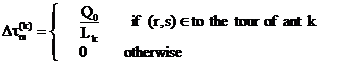
where Q₀ is a constant related to the amount of pheromone laid by ants and L_k is the tour length of the k-th ant.

The process is then iterated and the algorithm runs until some stopping criterion is met, a certain number of generations have been done or the average quality of the solution found by the ants of a generation has not changed for several generations.

ACO Applied on Optimal Power Flow

Our objective is to minimize the objective function of the OPF defined by (2), using into account the equality constraint (4), and the inequality constraint (5). The cost function implemented in ACO is defined as:

;

(10)

The search of the optimal parameters set is performed using into account a part of the equality constraints (4) which present the active power transmission losses (P_L) to be deal with in feasible region.

The search of the optimal control vector is performed which present the system transmission losses (P_L). These losses can be approximated in terms of B-coefficients as [23]:

(11)

These losses are represented as a penalty vector given by:

(12)

The transmission loss of a power System P_L can be calculated by the B-Coefficients method [24] and given by:

(13)

where Pg is a ng-dimensional column vector of the generator power of the units, Pg^T is the associate matrix of Pg, B is an ng×ng coefficients matrix, B₀ is an ng-dimensional coefficient column vector and B₀₀ is a coefficient.

Our objective is to search (Pg) set in their admissible limits to achieve the optimization problem of OPF. At initialization phase, (Pg) is selected randomly betweenand.

The use of penalty functions in many OPF solutions techniques to handle inequality constraints can lead to convergence problem due to the distortion of the solution surface. In this method only the active power of generators are used in the cost function. And the inequality constraints are scheduled in the load flow process. Because the essence of this idea is that the constraints are partitioned in two types of constraints, active constraints are checked using the ACO-OPF procedure and the reactive constraints are updating using an efficient Newton-Raphson Load flow procedure.

After the search goal is achieved, or an allowable generation is attained by the ACO algorithm. It is required to performing a load flow solution in order to make fine adjustments on the optimum values obtained from the ACO-OPF procedure. This will provide updated voltages, angles and transformer taps and points out generators having exceeded reactive limits. To determining ail reactive power of ail generators and to determine active power that it should be given by the slack generator using into account the deferent reactive constraints. Examples of reactive constraints are the min and the max reactive rate of the generators buses and the min and max of the voltage levels of all buses. All these require a fast and robust load flow program with best convergence properties. The developed load flow process is based upon the full Newton-Raphson algorithm using the optimal multiplier technique [25, 26].

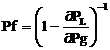
There are few parameters that to be set for the ant algorithm; these parameters are: ρ the evaporation rate, m the numbers of ants in the colony, α and β two coefficients. In the OPF case these values were obtained by a preliminary optimization phase, in which we found that the experimental optimal values of the parameters were largely independent of the problem. The initial pheromone τ₀ is given by τ₀ = (ng·L)-1 where L is the tour length produced by the nearest neighbor heuristic. The number of ants used is m=20. Regarding their initial positioning, ants are placed randomly, with at most one ant in each generator unit.

A local improvement method suggested by Johnson & McGeoch [27] called the restricted 3-opt method has been adapted for use in the ACO. It involves successive arc-exchanges in an attempt to improve a candidate solution. But we choose a limited number of exchanges in order to avoid over-long computation times. The local search is applied once the solution is built and the results of this phase are used to update the pheromone trails.

The Ant Colony Algorithm

Step1 Initialize:

Set t=0 {t is the time counter};

For every path (i,j) set an initial value τ_ij (t) and set Δτ_ij (t,t+n)= 0;

Place b_i(t) ants on every bus i {b_i(t) is the number of ants on bus i at time t}.

Set s=1 {s is the tabu list index};

For i=1 to n do;

For k=1 to b_i(t) do;

tabuk (s)= i {starting bus is the first element of the tabu list of the k-th ant}.

Step2 Repeat until tabu list is full {this step will be repeated (n-1) times}

Set s=s+1;

For i=1 to n do {for every bus};

For k=1 to b_i(t) do {for every k-th ant on bus i still not moved};

Choose the bus j to move to, with probability p_ij (t)

Move the k-th ant to j {this instruction creates the new values bj (t+1)}

Insert bus j in tabu k (s).

Step3 For k=1 to m do {for every ant}

Compute L^k {it results from the tabu list}

For s=1 to n-1 do {scan the tabu list of the k-th ant}

Set (h,l)=(tabuk (s),tabuk (s+1))

{[h, l] is the edge connecting bus s and s+1 in the tabu list of ant k}

L^K: represent the length crossed by the K-th ant.

Q: represent the amount of pheromone laid by the K-th ant.

Step4 For every edge (i,j) compute τ_ij(t+n)

Set t=t+n

For every path (i,j) set Δτ_ij(t,t+n)=0.

Step5 Memorize the shortest path found up to now

If (NC < NC_MAX ) or (not all the ants choose the same tour) {NC is the number of algorithm cycles in NC cycles are tested NCm tours} then;

Empty all tabu lists

Set s=1

For i=1 to n do

For k=1 to b_i(t) do

tabuk (s)=i {after a tour the k-th ant is again in the initial position}

Goto step 2

else

Print shortest tour and Stop.

Application Study, Results and Discussion

The ACO-OPF is coded in MATLAB environment version7.6 (R2008a), and run using an Intel Pentium 4, core duo 1.87 GHz PC with 2 Go DDRAM-II- and 2 Mo cache memory. All computations use real float point precision without rounding or truncating values. More than 6 small-sized test cases were used to demonstrate the performance of the proposed algorithm. Consistently acceptable results were observed.

The ACO-OPF method has been applied on the network test IEEE 57 buses that represent a portion of the American electric power system (the Midwestern, USA) for December 1961. This electric network is constituted of 57 buses and 7 generators (at the buses Nº: 1, 2, 3, 6, 8, 9 and 12) injecting their powers for a system nourishing 42 loads through 80 lines of transportation (Show in Fig 1). The base voltage for every bus is of 135 kV. Table 1 show the coefficients of the quadratic functions of cost and the limits min and max of the actives powers, the technical and economic parameters of the seven generators of the IEEE 57-bus electrical network.

Table 1: Generators parameters of the IEEE 57-bus Electrical Network

Bus Number	[MW]	[MW]	a [$/hr]	b [$/MWhr]	c [$/MW^2hr]
Bus 1	0.00	575.88	0.20	0.30	0.01
Bus 2	0.00	100.00	0.20	0.30	0.01
Bus 3	0.00	140.00	0.20	0.30	0.01
Bus 6	0.00	100.00	0.20	0.30	0.01
Bus 8	0.00	550.00	0.20	0.30	0.01
Bus 9	0.00	100.00	0.20	0.30	0.01
Bus 12	0.00	410.00	0.20	0.30	0.01

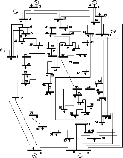
Figure 1. Topology of the IEEE 57-bus

Does have end to prove that the set of the three parameters of the colony of ants β, ρ and q0 is extensively independent of the problem of optimization to solve, we applied ACO-OPF on the network IEEE test 57 buses while using the 10 better combinations of the three parameters β, ρ and q0 and that give the best results for commercial traveler problem for the case of 30 cities [28]. The (Table 2) shows the values of actives powers, the losses of powers and the cost of fuel for the 10 ensemble wholes of parameters. We observe that all results are very near of the optimum. The average value of the cost for the 10 cases is the order of 3173.3126 $/h. The value min of the cost is 3172.202 $/h corresponds a (β = 10, ρ = 0.6 and        q0 = 0.3) with losses of powers 17.04 MWS. Therefore we remark that even the most distant cost value is acceptable since it is on the one hand moves away of the value min with only 0.056% and on the other hand the value of the losses corresponds has this value that is 17.04 MWS is better than the one corresponds at the value min with a report of 5.399%.

Table 2: Results of the ACO-OPF for the 10 ensemble wholes of parameters β, ρ and q0 for the IEEE 57-bus Electrical Network

Results	β = 10 ρ = 0.6 q0= 0.0	β = 11 ρ = 0.5 q0= 0.1	β = 9.5 ρ = 0.8 q0= 0.1	β = 10 ρ = 0.6 q0= 0.3	β = 12 ρ = 0.5 q0= 0.3
Pg1 [MW]	252.89	249.74	241.44	242.89	252.74
Pg2 [MW]	87.88	95.02	90.01	95.05	98.82
Pg3 [MW]	132.89	129.68	138.01	138.89	139.60
Pg6 [MW]	91.84	93.54	99.00	97.87	93.30
Pg8 [MW]	321.72	329.72	321.09	311.02	310.72
Pg9 [MW]	95.94	92.00	95.71	97.84	99.00
Pg12 [MW]	286.70	280.28	282.62	285.10	276.28
Power Loss [MW]	19.0600	19.1800	17.0800	17.9600	19.6600
Generation cost [$/hr]	3173.012	3173.106	3172.995	3172.202	3173.220
Results	β =9 ρ = 0.4 = 0.4	β = 11 ρ = 0.8 = 0.0	β = 10 ρ = 0.8 = 0.6	β = 6 ρ = 0.3 = 0.7	β = 11 ρ = 0.4 = 0.4
Pg1 [MW]	249.72	259.11	252.56	254.37	258.21
Pg2 [MW]	97.57	93.20	92.40	89.54	88.99
Pg3 [MW]	137.85	135.98	136.98	131.85	130.98
Pg6 [MW]	97.81	99.00	98.30	95.81	95.08
Pg8 [MW]	311.09	300.09	315.72	320.04	320.28
Pg9 [MW]	97.71	99.61	99.03	98.78	95.71
Pg12 [MW]	278.62	282.62	272.85	280.62	281.62
Power Loss [MW]	19.5699	18.8099	17.0400	20.2099	20.0699
Generation cost [$/hr]	3173.654	3173.007	3174.010	3173.995	3173.925

Results deliberate by ACO-OPF that corresponds at ensemble (β = 10, ρ = 0.6 and q0 = 0.3) are compare with those find by the QN method using the formula Update of BFGS and iterated with load flow of Newton Raphson (NR). The QN method uses a vector of penalty associates with the vector of controls Pgi. The values of the penalty coefficients are based on the formula of the B-coefficients losses. The use of the penalty functions that serves has keep the reactive powers of PV-bus in their admissible limits can produce problems of convergence that are practically has the distortion of the solution surface.

The constraints of security are also verified for the angles and the amplitudes of tensions, the levels of voltage (Per Unit) for the IEEE 57-bus Electrical Network are drawn in the Fig. 2. In ACO-OPF, we not make recourse for functions of penalty being given that only the actives powers of the generators are used in the selective function and the reactive powers are planned in the process of load flow. The essential of this idea is that the constraints are shared in two types: the active constraints that are verified by the procedure of ACO whereas the reactive constraints are update while using a procedure efficient of load flow by Newton-Raphson.

The results gotten including the generated cost and the losses of powers are compare with those acquired by the QN approved method and present on the Table 3.

Table 3: Comparison of the results gotten by ACO-OPF and QN-OPF on the IEEE 57-bus Electrical Network

Results	Min limit	Max limit	QN-OPF	ACO-OPF
Pg1 [MW]	0.00	575.88	275.41	242.89
Pg2 [MW]	0.00	100.00	98.95	95.05
Pg3 [MW]	0.00	140.00	137.75	138.89
Pg6 [MW]	0.00	100.00	99.27	97.87
Pg8 [MW]	0.00	550.00	289.97	311.02
Pg9 [MW]	0.00	100.00	99.05	97.84
Pg12 [MW]	0.00	410.00	267.56	285.10
Power Loss [MW]			17.16	17.9600
Generation cost [$/hr]			3175. 506	3172.202

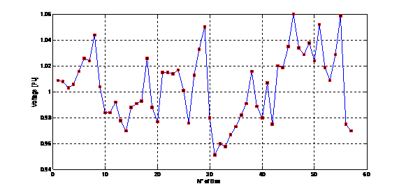
Figure 2. The levels of voltage (Per Unit) for the IEEE 57-bus Electrical Network

The ACO-OPF method is also compared with the evolutionary methods of the references [29]. The publication Younes M., Rahli M. and Koridak L.A. [29] present the optimal power flow based on hybrid genetic algorithm. A comparison between the generate active powers calculated by the ACO and the evolutionary methods as well as the costs, the losses of active power and the time of convergence has been illustrated in the Table 4.

Table 4: Comparison of the ACO-OPF with different evolutionary methods of optimization viewpoint cost, losses and times of convergence

Results	Min limit	Max limit	GA-OPF [29]	ACO-OPF
Pg1 [MW]	0.00	575.88	266.850	242.89
Pg2 [MW]	0.00	100.00	100.000	95.05
Pg3 [MW]	0.00	140.00	140.000	138.89
Pg6 [MW]	0.00	100.00	100.000	97.87
Pg8 [MW]	0.00	550.00	280.438	311.02
Pg9 [MW]	0.00	100.00	100.000	97.84
Pg12 [MW]	0.00	410.00	281.875	285.10
Power Loss [MW]			3171.785	3172.202
Generation cost [$/hr]			18.40	17.96
Time [Sec]			97.75	61.07

It is important to note that the gotten results are similar those given by the evolutionary programming. Since the difference between the cost values resulting from the ACO-OPF only defers of the GA-OPF by a rate of 0.08% and of the EP-OPF by a rate of 0.013%. The value of the losses found by ACO-OPF that is of 17.96 MWS is lower than the one found with GA-OPF by a rate of 1.85% and higher of the one of the EP-OPF by a rate of 2.449%. We add that the ACO-OPF is important to underline that the computer time for our method is better than the two other evolutionary methods.

Conclusions

In this paper, a novel ant colony optimization based approach to OPF problem has been presented. The proposed approach utilizes the global and local exploration capabilities of ACO to search for the optimal settings of the control variables. Different objective functions have been considered to minimize the fuel cost, to improve the voltage profile, and to enhance voltage stability. The proposed approach has been tested and examined with different objectives to demonstrate its effectiveness and robustness. The results using the proposed approach were compared to those reported in the literature. The results confirm the potential of the proposed approach and show its effectiveness and superiority over the classical techniques and genetic algorithms.

References

1. Dommel H.W., Tinney W.F., Optimal Power Flow Solutions, IEEE Transactions on power apparatus and systems, vol. PAS.87, No. 10, p. 1866-1876, 1968.

2. Bouktir T., Belkacemi M., Zehar K., Optimal power flow using modified gradient method, Proceedings ICEL’2000, U.S.T. Oran, Algeria, p. 436-442, 2000.

3. Fletcher R., Practical Methods of Optimization, John Willey & Sons, 1986.

4. Dorigo M., Optimization, learning, and natural algorithms, Ph.D. Dissertation (in Italian), Dipartimento di Elettronica, Politecnico di Milano, Italy, 1992.

5. Dorigo M., Di Caro G., The ant colony optimization metaheuristic, in Corne D., Dorigo M., Glover F., New Ideas in Optimization, McGraw-Hill, p. 11-32, 1997.

6. Dorigo M., Di Caro G., Gambardella L. M., Ant algorithms for discrete optimization, Artificial Life, Vol. 5, No. 2, p. 137-172, 1999.

7. Dorigo M., Maniezzo V., Colorni A., Ant System, optimization by a colony of cooperating agents, IEEE Trans. System Man. and Cybernetics, Part B: Cybernetics, Vol. 26, No. 1, p. 29-41, 1996.

8. Dorigo M., Gambardella L. M., Ant colonies for the traveling salesman problem, BioSystems, Vol. 43, p. 73-81, 1997.

9. Dorigo M., Gambardella L. M., Ant colony System: a cooperative learning approach to the traveling salesman problem, IEEE Transactions on Evolutionary Computation, Vol. l, No. 1, p. 53-66, 1997.

10. Maniezzo V., Colorni A., The ant System applied to the quadratic assignment problem, IEEE Trans. Knowledge and Data Engineering, Vol. 11, No. 5, p. 769-778, 1999.

11. Stuetzle T., Dorigo M., ACO algorithms for the quadratic assignment problem, in Corne D., Dorigo M., Glover F., New Ideas in Optimization, McGraw-Hill, 1999.

12. Bullnheimer B., Haïti R. F., Strauss C., Applying the ant System to the vehicle routing problem, in Voss S., Martello S., Osman I. H., Roucairol C., MetaHeuristics: Advances and Trend in Local Search Paradigms for Optimization, Kluwer, p. 285-296, 1999.

13. Bullnheimer B., Haïti R. F., Strauss C., An improved ant System algorithm for the vehicle routing problem, Ann. Oper. Res., Vol. 89, p. 319-328, 1999.

14. Gambardella L. M., Taillard E., Agazzi G.: MACS-VRPTW a multiple ant colony System for vehicle routing problems with time Windows, in Corne D., Dorigo M., Glover F., New Ideas in Optimization, McGraw-Hill, p. 63-76, 1999.

15. Di Caro G., Dorigo M., Ant colonies for adaptive routing in packet-switched communication networks, Proc. 5th Int. Conf. Parallel Problem Solving From Nature, Amsterdam, The Netherlands, p. 673-682, 1998.

16. Costa D., Hertz A., Ants can color graphs, J. Oper. Res. Soc., Vol. 48, p. 295-305, 1997.

17. Schoofs L., Naudts B., Ant colonies are good at solving constraint satisfaction problems, Proc. 2000 Congress on Evolutionary Computation, San Diego, CA, p. 1190-1195, 2000.

18. Wagner I. A., Bruckstein A. M., Hamiltonian(t)-an ant inspired heuristic for recognizing Hamiltonian graphs, Proc. 1999 Congress on Evolutionary Computation, Washington, D.C., p. 1465-1469, 1999.

19. Bauer A., Bullnheimer B., Hartl R. F., Strauss C., Minimizing total tardiness on a single machine using ant colony optimization, Central Eur. J. Oper. Res., Vol. 8, No. 2, p. 125-141, 2000.

20. Colorni A., Dorigo M., Maniezzo V., Trubian M., Ant system for job-shop scheduling, Belgian J. Oper. Res., Statist. Comp. Sci. (JORBEL), Vol. 34, No. 1, p. 39-53, 1994.

21. Den Besteb M., Stützle T., Dorigo M., Ant colony optimization for the total weighted tardiness problem, Proc. 6th Int. Conf. Parallel Problem Solving from Nature, Berlin, p. 611-620, 2000.

22. Merkle D., Middendorf M., An ant algorithm with a new pheromone evaluation rule for total tardiness problems, Proceedings of the EvoWorkshops 2000, Berlin, Germany: Springer-Verlag, Vol. 1803 then Lecture Notes in Computer Science, p. 287-296, 2000.

23. Wood A. J., Wollenberg B.F., Power Generation, Operation and Control, 2nd Edition, John Wiley, 1996.

24. Del Toro V., Electric Power Systems, Vol. 2, Prentice Hall, Englewood Cliffs, New Jersey, USA, 1992.

25. Stagg G. W., El Abiad A. H., Computer methods in power systems analysis, McGraw Hill International Book Company, 1968.

26. Kumar S., Billinton R., Low bus voltage and ill-conditioned network situation in a composite system adequacy evaluation, IEEE Transactions on Power Systems, Vol. PWRS-2, No. 3, 1987.

27. Johnson D.S., McGeoch L.A., The traveling salesman problem: a case study in local optimization, in E. H. L. Aarts, J. K. Lenstra: Local Search in Combinatorial Optimization, John Wiley and Sons, p. 215-310, 1997.

28. Gaertner D., Natural Algorithms for Optimisation Problems,’ Final Year Project Report’ June 20, 2004.

29. Younes M., Rahli M., Koridak L.A., Optimal Power Flow Based on Hybrid Genetic Algorithm, Journal of Information Science and Engineering, Vol. 23, pp. 1801-1816, 2007.

30. Wood A. J., Wollenberg B. F., Power Generation, Operation and Control, New York, John Wiley and Sons, 1984.

31. Chowdhury B. H., Rahman S., A Review Of Recent Advances In Economic Dispatch, IEEE Transactions on Power Systems, Vol. 5, No. 4, pp. 1248-1259, 1990.