Economic Dispatch for Power System included Wind and Solar Thermal energy
Saoussen BRINI, Hsan Hadj ABDALLAH, and Abderrazak OUALI
ENIS, Dép. Génie Electrique, 3038 Sfax, Tel.:74 274 088
E-mails: ingenieurbrini@yahoo.fr, hsan.haj@enis.rnu.tn, abderrazak.ouali@enis.rnu.tn
Abstract
With the fast development of technologies of alternative energy, the electric power network can be composed of several renewable energy resources. The energy resources have various characteristics in terms of operational costs and reliability. In this study, the problem is the Economic Environmental Dispatching (EED) of hybrid power system including wind and solar thermal energies. Renewable energy resources depend on the data of the climate such as the wind speed for wind energy, solar radiation and the temperature for solar thermal energy. In this article it proposes a methodology to solve this problem. The resolution takes account of the fuel costs and reducing of the emissions of the polluting gases. The resolution is done by the Strength Pareto Evolutionary Algorithm (SPEA) method and the simulations have been made on an IEEE network test (30 nodes, 8 machines and 41 lines).
Keywords
economic dispatch, total cost, active losses, multi objectives optimization, evolutionary algorithms, SPEA, renewable energy
Introduction
The economic and environmental problems in the power generation have received considerable attention. The apparition of the energy crisis and the excessive increase of the consumption have obliged production companies to implant renewable sources. However, this production poses many technical problems for their integration in the electric system.
The economic dispatch [8, 16] is a significant function in the modern energy system. It consists in programming correctly the electric production in order to reduce the operational cost [4, 7, 10, 15]. Recently, the wind power and solar thermal power attracted much attention like promising renewable energy resources [1, 6, 11, 18, 19, 22].
The problem is formulated as a multiobjective optimization problem [3, 5, 9, 24, 25]. It consists in distributing the active and renewable productions between the power stations of the most economic way, to reduce the emissions of the polluting gases and to maintain the stability of the network after penetration of renewable energy. The number of decision variables of the problem is related to all the nodes of the network.
Renewable energy
In this study, it is interested in two types of energies; wind power and thermal solar energy.
Wind energy
The mechanical power recovered by a wind turbine can be written in the form [6, 17, 23]:
|
|
(1) |
where CP, is the aerodynamic coefficient of turbine power (it characterizes the aptitude of the aerogenerator to collect wind power), ρ is the air density, Rp the turbine ray and VW wind speed. The power coefficient value CP, depends on the rotation speed of turbine and wind speed.
Mechanical adjustment of the wind power
Wind turbine is dimensioned to develop a nominal power Pn from a nominal wind speed Vn. For wind speeds higher than Vn, the wind mill must modify these aerodynamic parameters in order to avoid the mechanical overloads, so that the power recovered by the turbine does not exceed the nominal power for which the wind mill was designed.
Figure 1. Diagram of the useful power according to the wind speed.
According to the figure1, the characteristic of power according to the wind speed comprises four zones. Zone 1, where Pw = 0, zone 2, in which useful power depends on wind speed. Vw, zone 3, generally where provided power Pw remains appreciably equal to Pn and finally zone 4,Pw = 0
Solar energy
Solar energy is energy produced by the solar radiation, directly or in a diffuse way through the atmosphere. Thanks to various processes, it can be transformed into another form of useful energy for the human activity, in particular in electricity or heat [14, 17, 23].
The maximum power provided by a solar panel is given by the following characteristic [14, 17]:
|
|
(2) |
Ec is solar radiation, Tjref is the reference temperature of the panels of 25°C, Tj is the cells junction temperature (°C), P1 represent the characteristic dispersion of the panels and the value for one panel is included enters 0.095 to 0.105 and the parameter P2=-0.47%/C°; is the drift in panels temperature [14].
The addition of one parameter P3 to the characteristic, gives more satisfactory results:
|
|
(3) |
This simplified model makes it possible to determine the maximum power provided by a group of panels for solar radiation and panel temperature given, with only three constant parameters P1, P2 and P3 and simple equation to apply.
A thermal solar power station consists of a production of solar system of heat which feeds from the turbines in a thermal cycle of electricity production.
Formulation of problem
The control system problem can be treated as follows:
Of absence of the auxiliary
elements, the problem consists in extracting the maximum of power from the
renewable sources. Then, we slice this power of the total demand PD.
the remaining total demand![]() , will distributed between the thermal
power stations. The problem is reduced for a speed wind Vw and solar
radiation Ec given to minimize the thermal cost functions and the emissions of
polluting gases.
, will distributed between the thermal
power stations. The problem is reduced for a speed wind Vw and solar
radiation Ec given to minimize the thermal cost functions and the emissions of
polluting gases.
To approach to the reality, it is obvious that to must take account of the variation of the wind and solar radiation that can be done by using the techniques of the neurons networks which consists in forming a data base for various wind speed Vw, solar radiation Ec and total power demand PD. The neurons network is composed of three layers, the entries layer is formed by Vw, Ec et PD; the hidden internal layer which the number of neurons is variable and the exit layer which consists of 10 neurons which represent the minimal cost F1, the emissions of polluting gases F2, the generating nodes powers . The structure of this network is given by the figure (2).
Figure 2. Structure du réseau de neurones utilisé
Objective functions
Fuel cost function
The fuel cost function ![]() in $/h is
represented by a quadratic function as follow [2, 5, 19]:
in $/h is
represented by a quadratic function as follow [2, 5, 19]:
|
|
(4) |
The coefficients![]() ,
, ![]() and
and ![]() are
appropriate to every production unit,
are
appropriate to every production unit, ![]() is the real power output of i-th
generator and
is the real power output of i-th
generator and ![]() is the number of thermal generators.
is the number of thermal generators.
Emission fonction
The atmospheric emission can be represented by a function that links emissions with the power generated by every unit. The emission of SO2 depends on fuel consumption and has the same form as the fuel cost [8, 13].
The emission of NOx is difficult to predict and his production is associated to many factors as the temperature of the boiler and content of the air [12].
The emission function in ton/h which represents SO2 and NOx emission is a function of generator output and is expressed as follow [20]:
|
|
(5) |
Where![]() ,
,![]() and
and ![]() are the coefficients of
emission function corresponding to the i-th generator. These three
parameters are determined by adjustment techniques of curves based on reel
tests [13].
are the coefficients of
emission function corresponding to the i-th generator. These three
parameters are determined by adjustment techniques of curves based on reel
tests [13].
Problem constraints
The problem constraints are five types:
· Production capacity constraints
The generated real power of each generator at the bus i
is restricted by lower limit ![]() and upper limit
and upper limit![]() :
:
|
|
(6) |
· Power balance constraint
The total power generation and the wind power must cover
the total demand ![]() and the power loss p in
transmission lines, so we have:
and the power loss p in
transmission lines, so we have:
|
|
(7) |
· Active power loss constraint
Active power loss of the transmission and transport lines, are positives:
|
|
(8) |
· Renewable power constraint:
The renewable power used for dispatch should not exceed the 30% of total power demand:
|
|
(9) |
Thus, the problem to be solved is formulated as follow:
·
Minimize:(![]() )
)
Under:
|
|
Multi objectives Optimization
Principle
The multi-objective optimization problem is formulated in general as follow:
|
|
(10) |
with:
![]() : number of objectives functions
: number of objectives functions
![]() : number of equality and
inequality respectively constraints
: number of equality and
inequality respectively constraints
![]() : decision vector.
: decision vector.
Two solutions x1 and x2 of such optimization problem, we could have one which dominates the other or none dominates the other.
In a minimization problem, a solution x1 dominates other solution x2 if the following two conditions are satisfied:
|
|
(11) |
Define by ![]() the satisfiesability set, that is to say:
the satisfiesability set, that is to say: ![]()
where
![]() and
and ![]()
A decision
vector![]() is none dominated compared to a set
is none dominated compared to a set![]() , if:
, if:
|
|
(12) |
The optimize solutions set that are non-dominated within the entire search space are denoted as Pareto-optimal and the set of objectives vectors corresponding constitute the Pareto-optimal set or Pareto-optimal front.
SPEA approach (Strength Pareto Evolutionary Algorithm)
In [18], Zitzler and Thiele propose an elitist evolutionary approach to solve a multi objective problem which is called Strength Pareto Evolutionary Algorithm (SPEA). The Elitism is introduced by an external Pareto set. This set stores the non-dominated solutions funded during the resolution of the problem. In order to reduce the size of the external set, an average linkage based on hierarchical clustering algorithm is used without destroying the characteristics of the trade-off front.
Noting by:
P : the current population.
![]() : the external population.
: the external population.
![]() : the size
of current population.
: the size
of current population.
![]() the fitness of an individual i.
the fitness of an individual i.
![]() the strength of an individual i.
the strength of an individual i.
The assignment procedure to calculate the fitness values is the following:
·
Step 1: For each individual ![]() is assigned a reel value
is assigned a reel value ![]() called
strength.
called
strength. ![]() is
proportional to the number of individuals in the current population dominated
by the individual i in the external Pareto set. It can be calculated as
follows:
is
proportional to the number of individuals in the current population dominated
by the individual i in the external Pareto set. It can be calculated as
follows:
For an individual ![]()
|
|
(13) |

The strength of a Pareto solution is also its fitness: ![]()
·
Step 2: The fitness of an individual ![]() is the sum of the strengths of
all external Pareto individuals
is the sum of the strengths of
all external Pareto individuals ![]() dominated by
dominated by![]() . We add one in odder
to guarantee that Pareto solutions are most likely to be produced.
. We add one in odder
to guarantee that Pareto solutions are most likely to be produced.
|
|
(14) |
where ![]()
The clustering algorithm is described by the following steps:
·
Step 1: To initialise clustering set C; each individual ![]() constitutes
a distinct cluster:
constitutes
a distinct cluster:
|
|
(15) |

·
Step 2: if the number of cluster is lower or equal to maximum size of
external set (![]() ), go to step 5. Else, go to step 3.
), go to step 5. Else, go to step 3.
·
Step 3: Calculate the distance between each pair of clusters. The distance
dc between two clusters ![]() and
and ![]() is defined as the
average distance between two pairs of individuals from each cluster:
is defined as the
average distance between two pairs of individuals from each cluster:
|
|
(16) |
![]() and
and ![]() are respectively the numbers
of individuals in clusters
are respectively the numbers
of individuals in clusters ![]() and
and![]() .
.
·
Step 4: Find the pair of clusters corresponding to the minimal distance ![]() between
them. Combine into a large one
between
them. Combine into a large one ![]() and return to step 2.
and return to step 2.
· Step 5: Find the centroid of each cluster. Select the nearest individual in this cluster to the centroid as a representative individual and remove all other individuals from the cluster.
·
Step 6: Thus, the reduced Pareto set ![]() is computed by uniting
these representatives:
is computed by uniting
these representatives: ![]()
Numeric Simulations and Comments
Presentation of the test network
The structure of the test system is shown in fig.1.Appendix A1. It was derived from the standard IEEE 30-bus 6-generator test system while adding to him two renewable generators. The characteristics of the wind mill are presented in table 1. The values of the fuel and emission coefficients are given in table2. The lines data and bus data are given respectively in tables 1 and 2 in Appendix A1.
Table 1. Wind mill Data
|
Characteristics of the wind mill |
||||
|
propeller Diameter
|
blades number |
Surface swept |
chechmate Height |
Nominal wind speed Vn |
|
34 m |
3 |
1480 m2 |
45 m |
15 m/s |
|
Nominal characteristics of the asynchronous generator |
||||
|
Interlinked voltage
|
Current |
Frequency |
power Pn |
Cos φ |
|
660 V |
760 A |
50 Hz |
790 Kw |
0.91 |
|
Rs |
Rr |
Lσ |
Xm |
Rm |
|
0.00374 Ω |
0.00324 Ω |
0.23 mH |
5.8 mH |
83.85 Ω |
Table 2: Generator cost and emission coefficients
|
|
|
G1 |
G2 |
G3 |
G4 |
G5 |
G6 |
|
Cost |
a |
10 |
10 |
20 |
10 |
20 |
10 |
|
b |
200 |
150 |
180 |
100 |
180 |
150 |
|
|
c |
100 |
120 |
40 |
60 |
40 |
100 |
|
|
Emission |
|
4.091 |
2.543 |
4.258 |
5.326 |
4.258 |
6.131 |
|
|
-5.554 |
-6.047 |
-5.094 |
-3.550 |
-5.094 |
-5.555 |
|
|
|
6.490 |
5.638 |
4.586 |
3.380 |
4.586 |
5.151 |
|
|
|
2.0 10-4 |
5.0 10-4 |
1.0 10-6 |
2.0 10-3 |
1.0 10-6 |
1.0 10-5 |
|
|
|
2.857 |
3.333 |
8 |
2 |
8 |
6.667 |
Lower limit and upper limit of the generated real power of each generator at the bus it is shown by (17):
|
|
(17) |
Results and Comments
Implementation and test of the neurons network
The neurons network is used to calculate in real time the active production in the thermal generating nodes and of the renewable origins. The structure of this network is given by the figure (2).
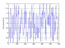
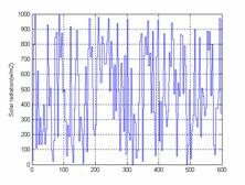
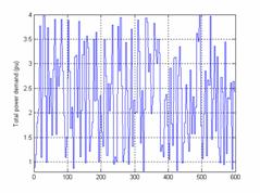
To ensure a good training of the neurons network, the base data is formed by 600 random solutions calculated by method SPEA and corresponding at a wind speed included enters 8 and 12 ms-1, solar radiation vary between 0w/m2 and 1000w/m2 and the total power demand vary between 0.8 and 4 pu.
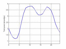
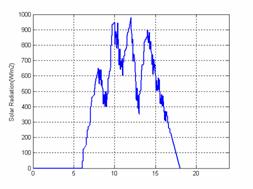
Training curves of wind speed, solar radiation and the total power demand are given by figures (3, 4 and 5).
|
|
|
|
Figure 3. Training curve of wind speed |
Figure 4. Training curve of solar radiation |
|
|
|
|
Figure 5. Training curve of total power demand |
|
During this phase, some of new examples are presented to the neurons network. The same examples were already simulated by SPEA method and we studied the quality of these answers given to table 3.
Table 3. Results of test neurons network
|
|
Test exemple |
||||||||||
|
Pw (pu) |
Ps (pu) |
Pg1 (pu) |
Pg2 (pu) |
Pg3 (pu) |
Pg4 (pu) |
Pg5 (pu) |
Pg6 (pu) |
Emiss (ton/h) |
Coût ($/h) |
||
|
PD1 |
2.35 |
0.6156 |
0.0475 |
0.3242 |
0.4352 |
0.4363 |
0.2052 |
0.3871 |
0.3795 |
0.1934 |
499.5495 |
|
PD2 |
3.43 |
0.7059 |
0.0175 |
0.4095 |
0.5220 |
0.5516 |
0.3635 |
0.5071 |
0.4846 |
0.1866 |
643.0993 |
|
PD3 |
3.35 |
0.8423 |
0.0385 |
0.3708 |
0.4870 |
0.5054 |
0.3575 |
0.4714 |
0.4605 |
0.1874 |
598.0519 |
|
PD4 |
1.16 |
0.3039 |
0.0252 |
0.3051 |
0.4284 |
0.4116 |
0.0939 |
0.3786 |
0.3598 |
0.1973 |
468.1725 |
|
PD5 |
0.93 |
0.2315 |
0.0412 |
0.3204 |
0.4743 |
0.4537 |
0.1231 |
0.3774 |
0.3504 |
0.1950 |
500.7442 |
|
PD6 |
1.25 |
0.3392 |
0.0301 |
0.3107 |
0.4249 |
0.4091 |
0.1017 |
0.3630 |
0.3410 |
0.1977 |
461.6945 |
|
PD7 |
2.65 |
0.4445 |
0.0266 |
0.3786 |
0.4834 |
0.5146 |
0.2245 |
0.4519 |
0.4197 |
0.1901 |
569.3929 |
|
PD8 |
3.10 |
0.5576 |
0.0388 |
0.4071 |
0.5251 |
0.5541 |
0.3173 |
0.5067 |
0.4879 |
0.1871 |
638.1037 |
|
|
Response of neurons network |
||||||||||
|
Pw (pu) |
Ps (pu) |
Pg1 (pu) |
Pg2 (pu) |
Pg3 (pu) |
Pg4 (pu) |
Pg5 (pu) |
Pg6 (pu) |
Emiss (ton/h) |
Coût ($/h) |
||
|
PD1 |
2.35 |
0.6156 |
0.0475 |
0.3202 |
0.4351 |
0.4317 |
0.2163 |
0.3874 |
0.3767 |
0.1932 |
499.6342 |
|
PD2 |
3.43 |
0.7059 |
0.0175 |
0.4105 |
0.5289 |
0.5448 |
0.3633 |
0.5111 |
0.4931 |
0.1864 |
643.0030 |
|
PD3 |
3.35 |
0.8423 |
0.0385 |
0.3711 |
0.4872 |
0.5114 |
0.3614 |
0.4711 |
0.4611 |
0.1872 |
598.8744 |
|
PD4 |
1.16 |
0.3039 |
0.0252 |
0.3054 |
0.4126 |
0.4144 |
0.1013 |
0.3814 |
0.3437 |
0.1995 |
466.2881 |
|
PD5 |
0.93 |
0.2315 |
0.0412 |
0.3199 |
0.4759 |
0.4538 |
0.1001 |
0.3633 |
0.3543 |
0.1951 |
501.1572 |
|
PD6 |
1.25 |
0.3392 |
0.0301 |
0.3106 |
0.4276 |
0.4097 |
0.1081 |
0.3665 |
0.3403 |
0.1972 |
463.4970 |
|
PD7 |
2.65 |
0.4445 |
0.0266 |
0.3652 |
0.4882 |
0.5168 |
0.2244 |
0.4543 |
0.4282 |
0.1901 |
569.3759 |
|
PD8 |
3.10 |
0.5576 |
0.0388 |
0.4019 |
0.5132 |
0.5537 |
0.3083 |
0.4982 |
0.4800 |
0.1875 |
637.9193 |
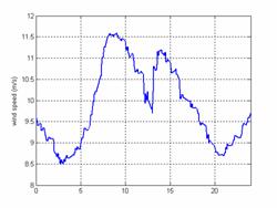
Figures (6, 7 and 8) present respectively the forecasts of wind speed, solar radiation and total power demand.
|
|
|
||
|
Figure 6. Forecast of wind speed |
Figure 7. Forecast of total power demand |
||
|
|
|
|
|
Figure 8.Forecast of solar radiation |
|
|
After the training phase of the neurons network, the simulation results are presented in the figures 9, 10, 11 and 12.
|
|
|
Figure 9. Power of the thermal generated nodes and PD’ |
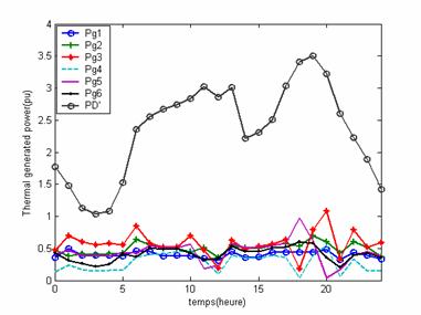
According to figure 9, we notice that the bus thermal generators powers remain variable within their limits.
Bus generator 2 has a remarkable participate by its active power Pg2 when total power demands P’Dis significant because it is the machine which has the more high cost.
|
|
|
Figure 10.Total power demand and renewable power |
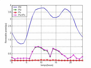
Figure 10; show the variation of solar thermal power, wind power and their resultant which remains lower than 30%of the total power demand PD.
|
|
|
|
Figure 11. Total cost function |
Figure 12. Emissions function |
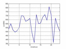
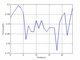
Figures 11 and 12 who represent respectively the variations of the total cost function and emissions of polluting gases function show that if the emissions of polluting gases decrease in the course of time then the total cost increases and conversely.
Conclusion
In this study we presented a method allowing the resolution of the problem of the Environmental Economic Dispatching of an electrical network including renewable energy sources. We made an optimization without auxiliary elements and the problem consists to extract the maximum of power from the renewable sources and to distribute the remainder of the power on the power stations. To have the solutions of the problem in real time we established them on a neurons network.
References
1. Granelli GP., Montagna M., Pasini GL., Marannino P., Emission constrained dynamic dispatch. Electr. Power syst. Res., 1992, PP. 56-64, 1992.
2. Farag A., Al-Baiyat S. and Cheng TC., 1995, Economic load dispatch multi objectives optimization procedures using linear programming techniques. IEEE Trans. On Power Syst., Vol. 10, No.2, PP. 731-738, 1995.
3. Abido M. A. and Bakhashwain J. M., 2005, Optimal VAR dispatch using a multiobjective evolutionary algorithm. Electrical power and energy systems, PP. 13-20, 2005.
4. Lin, C.E. and Viviani, G.L.. Hierarchical economic dispatch for piecewise quadratic cost functions, IEEE Transactions on Power Apparatus and Systems, Vol. 103, No. 6, pp. 1170-1175, 1984.
5. Abido M. A., 2003, A niched Pareto genetic algorithm for multi objectives environmental/economic dispatch. Electrical power and energy systems, PP. 97-105, 2003
6.Piwko, R., Osbom, D., Gramlich, R., Jordan, G., Hawkins, D., and Porter, K. (2005). Wind energy delivery issues, IEEE Power & Energy Magazine, November/December, pp. 67-56, 2005.
7. Lingfeng Wang and Chanan Singh., 2006, Tadeoff between Risk and Cost in Economic Dispatch Including Wind Power Penetration Using Praticle Swarm Optimisation. International Conference on Power System Technology, 2006.
8. Miranda, V. and Hang, P. S. (2005). Economic dispatch model with fuzzy constraints and attitudes of dispatchers, IEEE Transactions on Power Systems, Vol. 20, No. 4, Nov., pp. 2143-2145, 2005.
9. Wang, L. F. and Singh, C. Multi-objective stochastic power dispatch through a modified particle swarm optimization algorithm, Special Session on Applications of Swarm Intelligence to Power Systems, Proceedings of IEEE Swarm Intelligence Symposium, Indianapolis, May, pp. 127-135, 2006.
10. Zhao et al./ JZhejiang Univ SCI 2005. ‘Multiple objective particle swarm optimisation technique for economic load dispatch’ 6A(5) :420-427.
11. Hota, P. K. and Dash, S. K. (2004). Multiobjective generation dispatch through a neuro-fuzzy technique, Electric Power Components and Systems, 32: 1191-1206, 2004.
12. DeMeo, E. A., Grant, W., Milligan, M. R., and Schuerger, M. J. (2005). Wind plant integration: costs, status, and issues, IEEE Power & Energy Magazine, November/December, pp. 38-46, 2004.
13. Talaq J., El-Hawary F. and El-Hawary M., 1994, A summary of Environmental/Economic Dispatch Algorithms. Trans. On Power Systems, Vol. 6, No. 3, Aug 1994, pp. 1508-1516, 1994.
14. Faisal A. Mohamed, Heikki N. Koivo., (2007), Online Management of MicroGrid with Battery Storage Using Multiobjective Optimization, POWERENG 2007, April 12-14, Setubal, Portugal, 2007
15. Bhatnagar R. and Rahmen S., Dispatch of direct load control for fuel cost minimisation. IEEE Trans. on PS, Vol-PWRS-1, pp. 96-102,1986
16. Dhifaoui R., Hadj Abdallah H. et Toumi B., Le calcul du dispatching économique en sécurité par la méthode de continuation paramétrique. Séminaire à l’I.N.H.Boumerdes Algérie, 1987.
17. GERGAUD O., Modélisation énergétique et optimisation économique d'un système de production éolien et photovoltaïque couplé au réseau et associé à un accumulateur. Thèse de Doctorat de l’École Normale Supérieure de Cachan, 2002
18. Guesmi T., Hadj Abdallah H., Ben Aribia H. et Toumi A., Optimisation Multiobjectifs du Dispatching Economique / Environnemental par l’Approche NPGA.International Congress Renewable Energies and the Environment (CERE)’2005 Mars 2005, Sousse Tunisie, 2005.
19. D. B. Das and C. Patvardhan, ‘ New Multi-objective Stochostic Serch Technique for Economic Load Dispatch, ‘IEE Proc.-Gener. Transm. Distrib., Vol. 145,No. 6, pp.747-752, 1998.
20. Zahavi J., Eisenberg L., Economic–environmental power dispatch. IEEE Trans. Syst., Vol. 5, No. 5, 1985, PP. 485–489, 1985.
21. Warsono, D. J. King, and C. S. Özveren, Economic load dispatch for a power system with renewable energy using Direct Search Method, 1228-1233, 2007.
22. F. Li, JD. Pilgrim, C. Dabeedin, A. Chebbo, and RK. Aggarwal, “Genetic Algorithms for Optimal Reactive Power Compensation on the National Grid System”, IEEE Trans.Power Systems, vol. 20, n° 1, pp. 493-500, February 2005.
23. Lingfeng Wang, Chanan Singh, 2007, Compromise Between Cost and Reliability in Optimum Design of An Autonomous Hybrid Power System Using Mixed-Integer PSO Algorithm, Department of Electrical and Computer Engineering Texas A&M University
24. T. BOUKTIR, L. SLIMANI and M. BELKACEMI “A Genetic Algorithm for Solving the Optimal Power Flow Problem”, Leonardo Journal of Sciences, Issue 4, January-June p. 44-58, 2004.
25. Benjamin Baran, Member, IEEE, José Vallejos, Rodrigo Ramos and Ubaldo Fernandez, Member, IEEE. ‘Reactive Power Compensation using a Multi-objective Evolutionary Algorithm’ PPt 2001, IEEE Porto Power Tech Conference, 10th-13th September, Porto, Portugal.
26. Mohammad Taghi Ameli, Saeid Moslehpour, Mehdi Shamlo, Economical load distribution in power networks that include hybrid solar power plants, Electric Power Systems Research 78 1147–1152, 2008.
Appendix

Figure 1. Single-line diagram of IEEE 30-bus test system with two renewable power stations
Table 1. Line data
|
Line N° |
Connection |
Impedance (p.u.) |
Line N° |
Connection |
Impedance (p.u.) |
|
1 |
30-29 |
0.0192 + j0.0575 |
22 |
13-12 |
0.0192 + j0.0575 |
|
2 |
30-24 |
0.0452 + j0.1852 |
23 |
12-11 |
0.0452 + j0.1852 |
|
3 |
29-23 |
0.0570 + j0.1737 |
24 |
19-11 |
0.0570 + j0.1737 |
|
4 |
24-23 |
0.0132 + j0.0379 |
25 |
19-14 |
0.0132 + j0.0379 |
|
5 |
29-28 |
0.0472 + j0.1983 |
26 |
19-10 |
0.0348 + j0.0749 |
|
6 |
29-22 |
0.0581 + j0.1763 |
27 |
19-9 |
0.0727 + j0.1499 |
|
7 |
23-22 |
0.0119 + j0.0414 |
28 |
10-9 |
0.0116 + j0.0236 |
|
8 |
28-21 |
0.0460 + j0.1160 |
29 |
16-8 |
0.1000 + j0.2020 |
|
9 |
22-21 |
0.0267 + j0.0820 |
30 |
9-7 |
0.1150 + j0.1790 |
|
10 |
22-27 |
0.0120 + j0.0420 |
31 |
8-7 |
0.1320 + j0.2700 |
|
11 |
22-20 |
j0.2080 |
32 |
7-6 |
0.1885 + j0.3292 |
|
12 |
22-19 |
j0.5560 |
33 |
6-5 |
0.2544 + j0.3800 |
|
13 |
20-26 |
j0.2080 |
34 |
6-4 |
0.1093 + j0.2087 |
|
14 |
23-18 |
j0.2560 |
35 |
3-4 |
j0.3960 |
|
15 |
18-25 |
j0.1400 |
36 |
4-2 |
0.2198 + j0.4153 |
|
16 |
18-17 |
0.1231 + j0.2559 |
37 |
4-1 |
0.3202 + j0.6027 |
|
17 |
18-16 |
0.0662 + j0.1304 |
38 |
2-1 |
0.2339 + j0.4533 |
|
18 |
18-15 |
0.0945 + j0.1987 |
39 |
27-3 |
0.0636 + j0.2000 |
|
19 |
17-16 |
0.2210 + j0.1997 |
40 |
22-3 |
0.0169 + j0.0599 |
|
20 |
15-14 |
0.0824 + j0.1923 |
41 |
20-19 |
j0.1100 |
|
21 |
16-13 |
0.1070 + j0.2185 |
Table 2. Bus data
|
Line N° |
Type |
Active power (p.u) |
Reactive power (p.u) |
Bus voltage (p.u) |
Line N° |
Type |
Active power (p.u) |
Reactive power (p.u) |
Bus voltage (p.u) |
|
1 |
P-Q |
0.106 |
0.019 |
- |
16 |
P-Q |
0.082 |
0.025 |
- |
|
2 |
P-Q |
0.024 |
0.009 |
- |
17 |
P-Q |
0.062 |
0.016 |
- |
|
3 |
P-Q |
0.000 |
0.000 |
- |
18 |
P-Q |
0.112 |
0.075 |
- |
|
4 |
P-Q |
0.000 |
0.023 |
- |
19 |
P-Q |
0.058 |
0.020 |
- |
|
5 |
P-Q |
0.035 |
0.000 |
- |
20 |
P-Q |
0.000 |
0.000 |
- |
|
6 |
P-Q |
0.000 |
0.000 |
- |
21 |
P-Q |
0.228 |
0.109 |
- |
|
7 |
P-Q |
0.087 |
0.067 |
- |
22 |
P-Q |
0.000 |
0.000 |
- |
|
8 |
P-Q |
0.032 |
0.016 |
- |
23 |
P-Q |
0.076 |
0.000 |
1.010 |
|
9 |
P-Q |
0.000 |
0.000 |
- |
24 |
P-Q |
0.024 |
0.000 |
1.010 |
|
10 |
P-Q |
0.175 |
0.112 |
- |
25 |
P-V |
0.000 |
0.000 |
1.071 |
|
11 |
P-Q |
0.022 |
0.007 |
- |
26 |
P-V |
0.000 |
0.000 |
1.082 |
|
12 |
P-Q |
0.095 |
0.034 |
- |
27 |
P-V |
0.300 |
- |
1.010 |
|
13 |
P-Q |
0.032 |
0.009 |
- |
28 |
P-V |
0.942 |
- |
1.010 |
|
14 |
P-Q |
0.090 |
0.058 |
- |
29 |
P-V |
0.217 |
- |
1.045 |
|
15 |
P-Q |
0.035 |
0.018 |
- |
30 |
Bilan |
0.000 |
0.000 |
1.060 |