Clustering of the Self-Organizing Map based Approach in Induction Machine Rotor Faults Diagnostics
Tarek AROUI*, Yassine KOUBAA* and Ahmed TOUMI
Research Unity of Industrial Process Control (UCPI), National Engineering School of Sfax (ENIS), B.P.: W 3038 Sfax, Tunisia
E-mail(s): tarek.aroui@eniso.rnu.tn, yassine.koubaa@enis.rnu.tn,
Abstract
Self-Organizing Maps (SOM) is an excellent method of analyzing multidimensional data. The SOM based classification is attractive, due to its unsupervised learning and topology preserving properties. In this paper, the performance of the self-organizing methods is investigated in induction motor rotor fault detection and severity evaluation. The SOM is based on motor current signature analysis (MCSA). The agglomerative hierarchical algorithms using the Wards method is applied to automatically dividing the map into interesting interpretable groups of map units that correspond to clusters in the input data. The results obtained with this approach make it possible to detect a rotor bar fault just directly from the visualization results. The system is also able to estimate the extent of rotor faults.
Keywords
Induction motors; Broken rotor bars; Self-Organizing Maps; Clustering.
Introduction
The use of induction motors in todays industry is extensive due to their simplicity of construction, robustness and high efficiency. In addition, the progress in power electronics, control circuits and automatic have contributed to an increasing use of induction motors in the applications at variable speed. Whatever its use, the induction motors can be the seat of an important variety of failures.
Common failures occurring in induction motors can be classified as follows: Internal motor faults (short circuit of motor leads, inter-turn short circuits, ground faults, broken rotor bar, broken end-ring, bearing failures), and external motor faults (phase failure, asymmetry of main supply, ). In certain cases, the failures can be due to the whole drive (gearbox fault, shaft misalignment, ). These incipient faults, or gradual deterioration, can lead to motor failure if left undetected. Early fault detection allows to minimize downtime and to schedule adequate maintenance action.
Many researchers have focused their attention on incipient fault detection and preventive maintenance in recent years. Generally, two methods (invasive and non-invasive) for machine fault detection are distinguished. The non-invasive methods received a considerable attention because they are based on easily accessible and inexpensive measurements to diagnose the machine conditions without disintegrating the machine structure.
Recently, Artificial Intelligence (AI) techniques have been proposed for the non-invasive machine fault detection [1]. These AI-based techniques include expert systems, neural network, fuzzy logic and pattern recognition. Employs these techniques provides significant possibilities to overcome the limits of the traditional methods.
In this paper, we present the clustering of the Self-Organizing Maps (SOM) based tools for motor rotor faults detection and severity evaluation. SOM is trained and tested using experimental results on a real induction machine.
Broken rotor bar motor current signature
Generally, the diagnosis of induction motors focuses on the spectral analysis of the various temporal sizes of the induction machine (stator currents, magnetic fields, frame vibrations, rotational speed, ) to extract the faults indicators. In general, stator currents and voltages are preferred because they allow for the realization of non-invasive diagnostic systems. Motor Current Signature Analysis (MCSA) is the most widely used method. Thus, the current signature that is indicative of a broken rotor bars are the amplitude of the frequency components (1±2ks)fs.(Figure 1) and (k/p(1-s)±(1+2λ)s)fs where s is the slip and fs is the supply frequency [2].
Figure 1. Experimental healthy (---) and faulty (two broken rotor bars) stator current spectrum around fundamental
Clustering
Clustering is the unsupervised classification of objects into different groups. The objective of the clustering is to divide a set of data vectors into groups (or clusters) so that the degree of similarity between two vectors is maximal if they belong to the same group and minimal otherwise. Applied to the diagnosis of the asynchronous machine, classification must be able to distinguish the different operating conditions, with and without fault.
Hierarchical clustering
There are two major methods of clustering, hierarchical clustering and partative clustering. Hierarchical algorithms find successive clusters using previously established clusters. Hierarchical algorithms can be agglomerative ("bottom-up") or divisive ("top-down") to build a hierarchical clustering tree (dendrogram), which can be cut at any level to obtain a desired number of clusters. Agglomerative techniques are more commonly used, and this is the method considered in this paper.
Agglomerative algorithms begin with each element as a separate cluster and merge them into successively larger clusters. At each step, it seeks to minimize distances within and maximize distances between clusters.
In general, hierarchical clustering uses the Wards criterion [3]. Then, the union of every possible cluster pair (Ci et Cj) reduce the within-cluster distance by:
|
|
(1) |

where ni is the
number of samples in cluster Ci , ![]() is the Euclidean norm and gi is the centre of the cluster i.
is the Euclidean norm and gi is the centre of the cluster i.
Self-Organizing Map (SOM)
The Self-Organizing Map (also known as Kohonen map) is an unsupervised artificial neural network which is a powerful method for clustering and visualization of high-dimensional data [4].
The SOM algorithm implements a nonlinear topology preserving mapping from a high-dimensional input data space onto a low dimension discrete space (usually 1D,2D or 3D), called the topological map.
A map consists of m neurons (or units) located on a regular low dimensional grid, usually a two-dimensional rectangular or hexagonal grid, that defines their neighbourhood relationships. Each neuron C is represented by a weight vector Wc = [w1Λwd] where d is the dimension of the input vector [4].
Training of the SOM
During training procedure, the weight vectors are adapted in such a way that close observations in the input space would activate two close neurons of the SOM [5].
The SOM is trained iteratively. At each training step, a sample input data vectors X is randomly presented from the training data sets, and the distance between the data and all the weight vectors of the SOM is calculated. The neuron whose weight vector is closet to the input vector is called the best-matching unit, often denoted bmu:
|
|
(2) |

where wbmu is the best-matching unit weight vector.
After finding the bmu, the weight vectors of the SOM are updated. The weight vectors of the bmu and its topological neighbours are moved closer to the input data vector. The weight-updating rule of the unit i is:
|
|
(3) |
where t is time, e(t) is a learning rate and hbmu(i,t) is defined as the neighbourhood kernel function around the bmu. Usually, e(t) is a decreasing function of time and should be between 0 and 1. The Gaussian neighbourhood function is chosen:
|
|
(4) |

where s (t) is the neighborhood radius [6]:
|
|
(5) |

si and sf are the initial and final neighbourhood radius, T is the training length, rk Î Â2 and rj Î Â2 are position of neurons k et j on the map.
Labelling of the SOM
After the training phase, it is possible to use the SOM to construct a classifier in which each neuron represents one class type. The classifier can then assign to each data vectors the corresponding bmu cluster.
However, training of the self-organizing map is totally unsupervised. Therefore, it is not known what kind of data each of the obtained units represents.
If labelled data are available, this information can be used to assign each neuron a label. The SOM is labelled based on votes between the labels according input data vectors and only uses the one which is most frequent. Finally, class label of each original data vector is the label of the corresponding bmu [6].
Clustering of the SOM
When not enough labelled data is available, the previous approach did not work at all. Then, to facilitate analysis of the map and the data, similar units need to be grouped to reduce the number of clusters. This is due to the topological ordering of the unit maps. Several methods [7, 8] are often used to perform this task. We have chosen to apply agglomerative hierarchical algorithms using the Wards method to cluster our maps.
The clustered map can then be labelled. The primary benefit of this approach is to use more labelled data to assign each cluster a label and facilitate the analysis of revealed groups.
Experimental Setup
The characteristics of the three phase induction motor used in our experiment are 5.5.KW 220/380.V 20.6/11.9.A 50Hz 2875.rpm. The needed load of the induction motor was established by connecting the test motor to an eddy current brake via a flexible coupling (Figure 2).
In order to allow tests to be performed at different load levels, the brake DC supply current is controllable. A MATLAB Application Program Interface (API) is built to allow The ARCOM A/D PCI card to communicate directly with MATLAB.
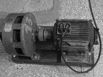
Figure 2. View of the experimental setup
A current Hall Effect sensor was placed in one of the line current cables and the sampling rate is 4 kHz. For our experimentations, the motor was tested with the healthy rotor and a faulty rotor with one and two broken bars for three different load conditions (respectively 50%, 75% and 100% of the full load). The bars were broken by drilling holes through them.
SOM for induction motor fault diagnosis
The collected data from experiment consist of 180 samples (60 representatives from each fault case and from the healthy case) and each data vector is labelled with the class it belongs. For the detection of rotor bar faults of an induction motor, 14 parameters that seemed to be the best indicators of the faults were taken in consideration: the amplitude of 10 frequency components centred on the fundamental and 4 components around 5th harmonic. Then, the database size is 180 × 14 data vectors, two thirds of them were used to train the SOM. The rest are left for testing the networks performance.
As the amplitude of the parameters is in different scales, the normalization process is important so that all variables will be equally important on the training result. Normalization of the variance of vector components to unity, and its mean to zero is employed in this paper.
A two-dimensional SOM of 55 neurons (11 by 5), organized in a hexagonal neighbourhood lattice, was trained using a SOM toolbox implemented in a free software Matlab-Package[1] SOM_PAK and developed in the Helsinki University of Technology.
Visualization of the SOM
The first step in the analysis of the map is visual inspection. In the following, the basic visualization of the SOM is introduced.
The Unified distance matrix (U-matrix) shown in Figure 3(a) is useful for detection of cluster borders and especially suitable for estimation of inter cluster distances. The U-matrix shows distances between neighbouring map units using grey levels. Dark gray represents long distances and light grey short ones. It is easy to see that the map unit in the top right corner is a very clear cluster.
The SOM do not utilise class information during the training phase. Class labels can be displayed an empty grid as a post-process after the completion of training. Figure 3(b) clearly identify the label associated with each map unit (N= healthy rotor, D=faulty rotor with one broken bar and S= faulty rotor with two broken bars). From the labels it can be seen that unlabeled units indicate cluster borders and the map unit in the top right corner corresponds to the normal operating condition. The two other operating conditions form the other cluster. The U-matrix shows no clear separation between them, but from the labels it seems that they correspond to two sub clusters.
Figure 4 plot shows the projection of both the training data set and the map grid. A principle component projection is made for the data, and applied to the map. Neighbouring map units are joining with lines to show the SOM topology. Labels associated with map units are also shown. From this figure one can see that the projection confirms the existence of two different clusters (Healthy and faulty rotor).
Also, visualization of the SOM shows that its impossible to isolate clearly the classification boundary in the faulty rotor case. However, increased of faulty level can be seen from the left bottom corner to right top corner of the Kohonen map. For further investigation, the map needs to be partitioned.
|
|
|
|
(a) |
(b) |
Figure 3. Visualization of the SOM: (a) U-matrix and (b) labelled map (N= healthy rotor, D=faulty rotor with one broken bar and S= faulty rotor with two broken bars).
Figure 4. The projection of both the training data set and the map grid ( ·- healthy rotor,
ê- faulty rotor with one broken bar and ¨- faulty rotor with two broken bars).
The agglomerative hierarchical algorithms using the Wards method is applied to cluster our maps. Figure 5(a) shows the dendrogram resulting of the clustering procedure. Hierarchical clustering tree seems to indicate that there are three clusters on the map (the dendrogram is cut where there is a large distance between two merged clusters).
Figure 5. (a) Dendrogram of the hierarchical algorithms
We can see in Figure 5(b) the final map and the clustering obtained. The analysis of each cluster is based on the labelled map:
§ The region 1 corresponds to the healthy motor,
§ The region 2 corresponds to the faulty rotor with one broken bar,
§ The region 3 corresponds to the faulty rotor with two broken bars.
Figure 5. (b) Clustering resulting of the hierarchical algorithms
Classification performance
In order to use the labelled map as an automatic classification tool for a data set. The main idea is to find, for each data sample, the best matching unit from the map. Then, the class label of that unit is given to the sample [5]. Clustering accuracy can be evaluated as fraction of correctly classified input samples. The classification performances of the SOM using the training and testing data sets are summarized in Tables 1 and 2, respectively. The figures in tables 1 and 2 outlined the number of times each map unit was the bmu.
The results indicate that the classification performance for the SOM is:
§ The tests carried out with a healthy normal condition activate almost only class number 1. We can notice that the SOM has 96.66% accuracy for the data with healthy normal condition.
§ Broken rotor bars are always distinguished from the healthy situation. Only 0.8% of all samples with rotor faults activate class number 1.
There are difficulties in distinguishing one broken rotor bar from two broken operation. However, in total, over 80% of all samples are correctly classified in all rotor fault situations.
Table 1. Classification performance of the SOM using training data set
|
|
|||
|
|
Activation of class number 1 (%) |
Activation of class number 2 (%) |
Activation of class number 3 (%) |
Healthy rotor |
9 |
5 |
0 |
|
Rotor with one broken bars |
0 |
75 |
25 |
|
Rotor with two broken bars |
0 |
30 |
70 |
Table 2. Classification performance of the SOM using test data set
|
|
|||
|
|
Activation of class number 1 (%) |
Activation of class number 2 (%) |
Activation of class number 3 (%) |
Healthy rotor |
100 |
0 |
0 |
|
Rotor with one broken bars |
4.3 |
78.3 |
17.4 |
|
Rotor with two broken bars |
0 |
10 |
90 |
Conclusions
In this paper, we have presented induction motor rotor fault detection and severity evaluation using Self Organising Maps (SOM). The SOM were trained and tested using real measurement data from stator currents signals. This study shows the visualization abilities of Self-Organizing Maps to classify the type of motor faults.
We have shown that the clustered SOM obtained by agglomerative hierarchical algorithms using the Wards method give interesting groups of map units and facilitate easy visualization and interpretation of motor faults.
The method used in this paper offers interesting possibilities to analysis the motor condition (with and without fault). The results obtained have proved the efficiency of SOMs for induction motor diagnosis.
Acknowledgements
The authors would like to thank SITEX Company who finances this work. They also wish to express their deep appreciation for the support rendered by the electrical department members.
References
1. Filippetti F., Franceschini G., Tassoni C., Vas P., AI techniques in induction machines diagnosis including the speed ripple effect, IEEE Transations on Industry Applications, 1998, 34(1), p. 98-108.
2. Aroui T., Koubaa Y., Toumi A., Magnetic Coupled Circuits Modeling of Induction Machines Oriented to Diagnostics, Leonardo Journal of Sciences, 2008, 13, p. 103-121.
3. Ward J. H., Hierarchical grouping to optimize an objective function, J. American Statistical Association, 1963, 58(301), p. 235-244.
4. Kohonen T., Self-Organizing Maps, Berlin, Edition Springer, 2001.
5. Vesanto J., Himberg J., Alhoniemi E., Parhankangas J., Self-organizing map in Matlab: the SOM Toolbox, In Proceedings of the Matlab DSP Conference 1999, Espoo, Finland, pp. 35-40, November 16-17, 1999.
6. Kohonen T., Hynninen J., Kangas J., Laaksonen J., SOM_PAK: The Self-Organizing Map Program Package, Technical Report A31, Helsinki University of Technology, 1996.
7. Samuelides M., Réseaux de neurones, une approche connexionniste de lIntelligence Artificielle, Edition TEKNEA, 1991.
8. Vesanto J., Alhoniemi E., Clustering of the self-organizing map, IEEE Transactions on Neural Networks, 2000, 11(3), p. 586-600.