Stability Analysis for Compliant Constant-Force Compression Mechanisms

Ikechukwu Celestine UGWUOKE

Department of Mechanical Engineering, Federal University of Technology, Minna, Nigeria

E-mail: ugwuokeikechukwu@yahoo.com

Abstract

Stability analysis in compliant mechanism (CM) design is of utmost importance. From a practical point of view, a CM that is unstable is of no significance (has no practical value). Three useful plots were considered in the evaluation of each of the dynamic models of nine configurations of compliant constant-force compression mechanisms (CCFCMs) for their stability characteristics, which includes the polar plot based on the Routh-Hurwitz stability criterion, the Bode plot, and the Nyquist diagram which considers stability in the real frequency domain. Frequency-domain stability criterion is very useful for determining suitable approaches to adjusting the CCFCM parameters in order to increase its relative stability. The results obtained show that the CCFCMs investigated do exhibit higher relative stability for higher values of damping ratio, and for zero damping ratio, all the CCFCMs investigated were unstable. The result also show that for the CCFCMs investigated to be stable, damping ratio must be greater than 0.03 (ξ > 0.03) and depending on what attributes are most desirable, the CCFCM parameters can be optimized to achieve the desired results. Nyquist criterion provides us with suitable information concerning the absolute stability and furthermore, can be utilized to define and ascertain the relative stability of a system.

Keyword

Stability characteristics, Routh-Hurwitz stability criterion, Bode plot, Nyquist diagram, Absolute stability, Relative stability.

Introduction

Stability analysis in compliant mechanism (CM) design is of utmost importance. From a practical point of view, a CM that is unstable is of no significance (has no practical value). A stable system is defined as a system with a bounded (limited) system response. That is, if the system is subjected to a bounded input or disturbance and the response is bounded in magnitude, the system is said to be stable. A stable system is a dynamic system with a bounded response to a bounded input [1]. The concept of stability can be illustrated by considering a right circular cone placed on a plane horizontal surface. If the cone is resting on its base and is tipped slightly, it returns to its original equilibrium position. This position and response are said to be stable. If the cone rest on its side and is displaced slightly, it rolls with no tendency to leave the position on its side. This position is designated as the neutral stability. On the other hand, if the cone is placed on its tip and released, it falls onto its side. This position is said to be unstable [1]. These three positions are illustrated in Figure 1. The discussion and determination of stability has occupied the interest of many engineers. Maxwell and Vishnegradsky were the first to consider the question of stability of dynamic systems. In the late 1800s, A. Hurwitz and E. J. Routh published independently a method of investigating the stability of linear systems. The Routh-Hurwitz stability method provides an answer to the question of stability by considering the characteristic equation of the system.

Figure 1. The Stability of a Cone

Using type-synthesis techniques, Murphy et al. [2], generated 28 possible CCFCM configurations that generate a constant output force for a wide range of input displacements. The 28 configurations consist of different arrangements of pin joints and flexible segments. These 28 configurations have been reduced to 15 viable configurations and are divided into 5 classifications based on the number of flexible segments and their location in each configuration. These classifications and configurations are illustrated in Figure 2 [3]. Howell et al. [4] carried out the dimensional synthesis of several of these configurations. Nine of the fifteen configurations presented in Figure 2 were investigated for their stability characteristics and the results obtained will demonstrate the significance of stability characteristics analysis in the design of CMs.

Figure 2. Fifteen configurations of the CCFCM

Stability analysis for CCFCM models

Every CCFCM presented in Figure 2 has essentially the same pseudo-rigid-body model (PRBM). Figure 3 shows the generalized PRBM of CCFCMs [5]. The characteristic equation in Laplace variable is written as:

Δ(s) = q(s) = ans^n + an-1s^n-1 + … + a1s + a0 = 0

(1)

To ascertain the stability of the system, it is necessary to determine whether any one of the roots of q(s) lies in the right half of the s-plane. Writing Eq(1) in factored form gives the following equation:

an(s-r1) (s-r2) … (s-rn) = 0

(2)

where r_i = i^th root of the characteristic equation.

Multiplying the factors together, we find that:

q(s) = ans^n-1 – an(r1+r2+ … + rn)s^n-1 + an(r1r2 + r2r3 + r1r3 + …)s^n-2 – an(r1r2r3 + r1r2r4 +…)s^n-3 + … + an(-1)^nr1r2r3…rn = 0

(3)

In other words, for an n^th-degree equation, we obtain:

q(s) = ans^n-1 – an(sum of all roots)s^n-1 +           + an(sum of the products of the roots taken 2 at a time)s^n-2 –            - an(sum of the roots taken 3 at a time)s^n-3 + … +            + an(-1)^n(product of all n roots) = 0

(4)

Figure 3. The CCFCM configuration Class 3A-n and its Pseudo-rigid-body model

Examining Eq(4) shows that all the coefficients of the polynomial must have the same sign if all the roots are in the left-hand plane. Also it is necessary that all the coefficients for a stable system be nonzero. These requirements are necessary but not sufficient. That is, we immediately know the system is unstable if they are not satisfied; yet if they are satisfied, we must proceed further to ascertain the stability of the system [1].

            The Routh-Hurwitz stability criterion is a necessary and sufficient criterion for the stability of linear systems. The method was originally developed in terms of determinants. The criterion is based on ordering the coefficients of the characteristic equation given below:

ans^n + an-1s^n-1 + … + a1s + a0 = 0

(5)

Into an array or schedule as follows:

(6)

Further rows of the schedule are then completed as follows:

(7)

Where

	(8)
	(9)
	(10)

and so on.

The algorithm for calculating the entries in the array can be followed on a determinant basis or by using the form of Eq(8). The Routh-Hurwitz stability criterion states that the number of roots of q(s) with positive real parts is equal to the number of changes in sign of the first column of the Routh array. This criterion requires that there be no changes in sign in the first column for a stable system. This requirement is both necessary and sufficient. Table 1 gives the summary of the Routh-Hurwitz stability criterion for up to a sixth-order characteristic equation.

The Routh-Hurwitz method is useful for investigating the characteristic equation expressed in terms of the complex variable. To investigate the stability of the system in the real frequency domain, that is, in terms of frequency response, the concept of gain margin and phase margin in the context of Bode plots and Nyquist diagrams is introduced. Frequency response analysis provides useful insights into stability and performance characteristics of the system. The gain margin is a measure of how much the system gain would have to be increased when the phase is = -180° for the locus of the loop transfer function of the system to pass through the (-1, 0) point (the limit of stability). The phase margin is a measure of the additional phase lag required to bring the system to the limit of stability. In other words, it is the angle between the point -1 and the vector of magnitude. Gain and phase stability margins are clearly illustrated in Figure 2 and can easily be determined from both the Bode plot and the Nyquist diagram. The frequency response of a system can readily be obtained experimentally by exciting the system with sinusoidal input signals. Furthermore, a frequency-domain stability criterion would be useful for determining suitable approaches to adjusting the parameters of a system in order to increase its relative stability.

Figure 4. Gain and phase stability margins

The Nyquist stability criterion (developed by Harry Nyquist in 1932), is defined in terms of the (-1, 0) point on the polar plot or the 0-sB, -180° point on the Bode diagram or log-magnitude-phase diagram. Proximity to this stability point is a measure of the relative stability of a system. The Nyquist stability criterion is based on a theorem in the theory of the function of a complex variable due to Cauchy known as Cauchy’s principle of argument. Cauchy’s theorem is concerned with mapping contours in the complex s-plane.

To determine the relative stability of a closed-loop system using the Nyquist stability Criterion, one must first investigate the characteristic equation of the system given by:

F(s) = 1+L(s) = 0

(11)

For a single-loop system:

L(s) = G(s)H(s)

(12)

For a multi-loop system, the characteristic equation is given by:

F(s) = Δ(s) = 1 - ∑Ln + ∑LmLq … = 0

(13)

where Δ(s) is the graph determinant

Table 1. The Routh-Hurwitz stability criterion

n	Characteristic Equation	Criterion
2	s^2 + bs + 1 = 0	b > 0
3	s^3 + bs^2 + cs + 1 =0	bc – 1 > 0
4	s^4 + bs^3 + cs^2 + ds + 1 = 0	bcd – d^2 – b^2 > 0
5	s^5 + bs^4 + cs^3 + ds^2 +es + 1 = 0	bcd + b – d^2 – b^2e > 0
6	s^6 + bs^5 + cs^4 + ds^3 +es^2 + fs + 1 = 0	(bcd + bf – d^2 – b^2e)e + b^2c – bd + bc^2f – f^2 + bfe +cdf > 0

Cauchy’s principle of argument is stated thus; If a contour Γ_s in the s-plane encircles the zeros Z and poles P of F(s) and does not pass through any poles or zeros of F(s) and the traversal is in the clockwise direction along the contour, the corresponding contour Γ_F in the F(s)-plane encircles the origin of the F(s)-plane N times in the clockwise direction, with N given by:

N = Z - P

(14)

A contour map is a contour or trajectory in one plane mapped or translated into another plane by a relation F(s). Nyquist stability Criterion is concerned with the mapping of the characteristic equation F(s) = 1 + L(s) and the number of encirclements of the origin of the F(s)-plane. Alternatively, we may define the function F^'(s) so that:

F^'(s) = F(s) – 1 = L(s)

(15)

The change of functions represented by Eq(15) is very convenient because L(s) is typically available in factored form, while [1 + L(s)] is not. Then the mapping of Γ_s in the s-plane will be through the function F^'(s) = L(s) into the L(s)-plane. In this case, the number of clockwise encirclements of the origin of the F(s)-plane becomes the number of clockwise encirclements of the (-1, 0) point in the F^'(s) = L(s) – plane because F^'(s) = F(s) – 1. The modified Nyquist criterion therefore has the following form; the number of unstable close-loop polesis equal to the number of unstable open-loop polesplus the number of encirclementsof the point (-1, 0) of the Nyquist plot of L(s), that is:

Z = P + N

(16)

Clearly if the number of poles of L(s) in the right-hand s-plane is zero (P = 0), we require for a stable system that, and the contour must not encircle the (-1, 0) point. Also, if P is other than zero, then we require for a stable system that, which means that we must have N = -P, or P counterclockwise encirclements. Gain and phase margins may be found from Bode plots as follows; locate the point where the gain is zero dB (unity gain) and project down onto the phase diagram. The phase margin is the margin between the phase plot and – 180°. Similarly, locate the point where the phase angle reaches ±180° and project this back to the gain plot. The gain margin is the margin between this point and the zero dB level. If the gain is increased until this is zero, the system becomes unstable.

Results and Discussion

In the evaluation of the dynamic model for its stability characteristics, three useful plots were considered which includes the polar plot based on the Routh-Hurwitz stability criterion shown in Figure 5, the Bode plot shown in Figure 6, and the Nyquist diagram which considers stability in the real frequency domain shown in Figure 7. Figure 5 shows the plot of the root locations of the characteristic equation for the CCFCM. Using Routh-Hurwitz stability approach, the condition for stability is that all the roots must lie in the left hand s-plane. As shown in Figure 5, it can be seen clearly that all the roots of the characteristic equation lie in the left hand s-plane which means that the poles of the transfer function for the CCFCM have negative real part and therefore shows that the CCFCM is a stable system. Figure 6 and 7 shows the Bode plot and the Nyquist diagrams for the CCFCM. The Nyquist diagram is simply based on using open loop performance to test for close loop stability. The system will be unstable if the locus of the transfer function for the system has unity value at a phase crossover of ±180°. Two relative stability indicators “Gain Margin” and “Phase Margin” may be determined from both the Bode plot and the Nyquist diagram. As shown in Figure 6, the gain and phase margins are labeled clearly on the Bode diagrams. Nyquist criterion provides us with suitable information concerning the absolute stability and furthermore, can be utilized to define and ascertain the relative stability of a system. Figure 6 show that the CCFCM has a gain and phase margin of 33.096 dB and 11.363 degree respectively, which shows that the system is relatively stable. This is demonstrated clearly in Figure 7, which shows that the locus of the loop transfer function of the CCFCM does not pass through the (-1, 0) point (the limit of stability). This further confirms that the CCFCM is a stable system and also depending on what attributes are most desirable, the CCFCM parameters can be optimized to achieve the desired results.

Table 2. CCFCM configuration Class 3A-n

Mechanism Parameters	Parameter Values
r2	90 mm
r3	120 mm
m2	0.026 kg
m3	0.037 kg
ms	0.087kg
b	25.4 mm
h1	0.38 mm
h2	0.38 mm
h3	0.38 mm
I1	1.1615∙10^-13 m^4
I2	1.1615∙10^-13 m^4
I3	1.1615∙10^-13 m^4
E	207 Gpa
l1	9.00 mm
l2	10.50 mm
l3	12.00 mm
K1	2.6714 Nm
K2	2.2897 Nm
K3	2.0035 Nm

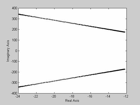
Figure 5. Plot of root locations of the characteristic equation of CCFCM model (ξ = 0.07)

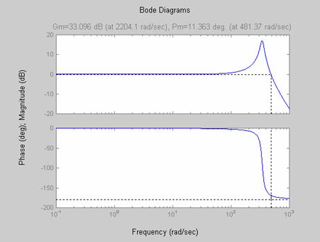
Figure 6. Bode diagram showing gain and phase margin (ξ = 0.07)

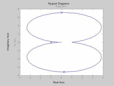
Figure 7. Nyquist diagram for the transfer function of the CCFCM model (ξ = 0.07)

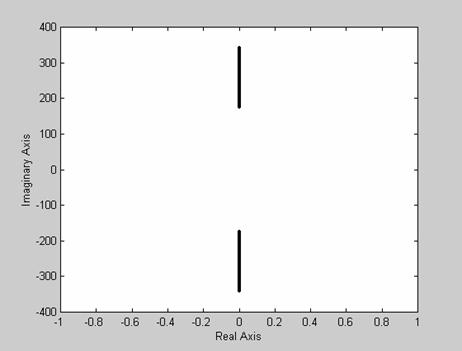
Figure 8. Plot of root locations of the characteristic equation of the CCFCM model (ξ = 0)

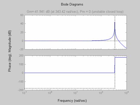
Figure 9. Bode diagram showing gain and phase margin (ξ = 0)

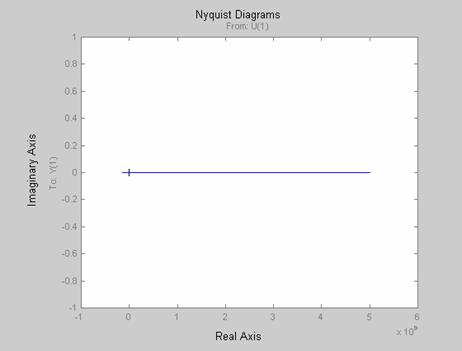
Figure 10. Nyquist diagram for the transfer function of the mechanism (ξ = 0)

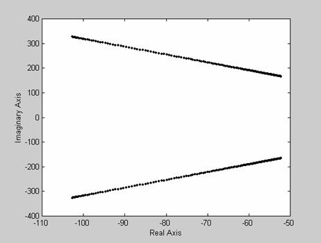
Figure 11. Plot of root locations of the characteristic equation of the CCFCM model (ξ = 0.3)

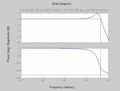
Figure 12. Bode diagram showing gain and phase margin (ξ = 0.3)

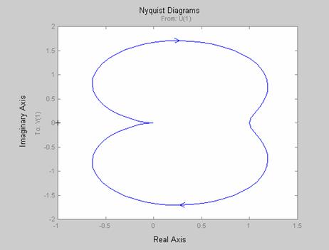
Figure 13. Nyquist diagram for the transfer function of the CCFCM model (ξ = 0.3)

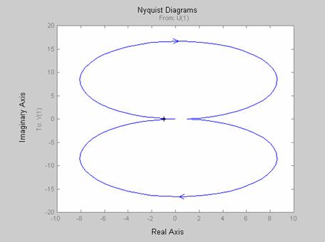
Figure 14. Nyquist diagram for the transfer function of the CCFM model (ξ = 0.03)

Table 3. Summary of stability results for all CCFCMs investigated

Mechanism Configuration	Gain Margin (dB)	Phase Margin (deg.)	Remark
Class 1A-a	34.251 (at 2244.7 rad/s)	11.363 (at 457.44 rad/s)	Stable System
Class 1A-b	28.157 (at 2015.3 rad/s)	11.363 (at 590.82 rad/s)	Stable System
Class 1B-e	34.458 (at 2251.8 rad/s)	11.363 (at 453.24 rad/s)	Stable System
Class 2A-h	41.754 (at 2461.4 rad/s)	11.363 (at 320.24 rad/s)	Stable System
Class 2A-i	31.043 (at 2128.2 rad/s)	11.363 (at 525.54 rad/s)	Stable System
Class 2B-j	37.290 (at 2342.9 rad/s)	11.363 (at 397.92 rad/s)	Stable System
Class 2B-k	30.568 (at 2110.1 rad/s)	11.363 (at 536.05 rad/s)	Stable System
Class 3A-n	33.096 (at 2204.1 rad/s)	11.363 (at 481.37 rad/s)	Stable System
Class 3A-o	41.861 (at 2463.8 rad/s)	11.363 (at 318.52 rad/s)	Stable System

Damping may be small, but its effect on the system stability and dynamic response, especially in the resonance region, can be significant [6]. To demonstrate this, we consider the stability of the CCFCM for zero damping. As shown in Figures 8 through 10, the CCFCM is unstable for zero damping. Also, considering the mechanism for a damping ratio of 0.3 as demonstrated in Figures 11 through 13, shows clearly that the CCFCM is relatively stable with a gain and phase margin of 33.401 dB and 50.209 degree respectively. This clearly demonstrates that the effect of damping on the CCFCM’s stability is highly significant. Comparing the results obtained for a damping ratio of 0.3 with that obtained for a damping ratio of 0.07 shows that the CCFCM gives better stability for higher damping ratios.

Table 4.Compliant Constant-Force Mechanism (CCFCM) Parameters and Values.

Parameter	Class 1A-a	Class 1A-b	Class 1B-e	Class 2A-h
r2	95.00 mm	80 mm	95.00 mm	120 mm
r3	80.00 mm	95 mm	95.00 mm	85 mm
m2	0.031 kg	0.028 kg	0.031 kg	0.037 kg
m3	0.028 kg	0.031 kg	0.031 kg	0.024 kg
ms	0.087 kg	0.087 kg	0.087 kg	0.087 kg
b	25.4 mm	25.4 mm	25.4 mm	25.4 mm
h1	0.38 mm	-	-	0.38 mm
h2	-	-	0.38 mm	0.38 mm
h3	-	0.38 mm	-	-
I1	1.1615 x 10^-13 m^4	-	-	1.1615 x 10^-13 m^4
I2	-	-	1.1615 x 10^-13 m^4	1.1615 x 10^-13 m^4
I3	-	1.1615 x 10^-13 m^4	-	-
E	207 Gpa	207 Gpa	207 Gpa	207 Gpa
l1	9.50 mm	-	-	12.00 mm
l2	-	-	9.50 mm	10.30 mm
l3	-	9.50 mm	-	-
K1	2.5308 Nm	-	-	2.0035 Nm
K2	-	-	2.5308 Nm	2.3456 Nm
K3	-	2.5308 Nm	-	-
Parameter	Class 2A-i	Class 2B-j	Class 2B-k	Class 3A-o
r2	85.00 mm	105.00 mm	85.00 mm	120.00 mm
r3	120.00 mm	85.00 mm	105.00 mm	90.00 mm
m2	0.024 kg	0.034 kg	0.024 kg	0.037 kg
m3	0.037 kg	0.024 kg	0.034 kg	0.026 kg
ms	0.087 kg	0.087 kg	0.087 kg	0.087 kg
b	25.4 mm	25.4 mm	25.4 mm	25.4 mm
h1	-	0.38 mm	0.38 mm	0.38 mm
h2	0.38 mm	-	-	0.38 mm
h3	0.38 mm	0.38 mm	0.38 mm	0.38 mm
I1	-	1.1615 x 10^-13 m^4	1.1615 x 10^-13 m^4	1.1615 x 10^-13 m^4
I2	1.1615 x 10^-13 m^4	-	-	1.1615 x 10^-13 m^4
I3	1.1615 x 10^-13 m^4	1.1615 x 10^-13 m^4	1.1615 x 10^-13 m^4	1.1615 x 10^-13 m^4
E	207 Gpa	207 Gpa	207 Gpa	207 Gpa
l1	-	10.50 mm	8.50 mm	12.00 mm
l2	10.30 mm	-	-	10.50 mm
l3	12.00 mm	8.50 mm	10.50 mm	9.00 mm
K1	-	2.2897 Nm	2.8285 Nm	2.0035 Nm
K2	2.3456 Nm	-	-	2.2897 Nm
K3	2.0035 Nm	2.8285 Nm	2.2897 Nm	2.6714 Nm

As demonstrated in Figures 5 through 13, an increase in the value of damping ratio from 0.07 to 0.3 increased the gain and phase margin from 33.096 dB and 11.363 degree to 33.401 dB and 50.209 degree respectively. Figure 14 shows that for the CCFCMs investigated to be stable, damping ratio must be greater than 0.03 (ξ > 0.03). Table 4 shows the mechanism parameters for the eight additional CCFCMs investigated and the results obtained for all the CCFCMs investigated have been summarized and presented in Table 3.

Conclusions

Stability analysis in CM design is of utmost importance. From a practical point of view, a CM that is unstable has no practical value. Three useful plots were considered in the evaluation of each of the dynamic models for their stability characteristics, which includes the polar plot based on the Routh-Hurwitz stability criterion, the Bode plot, and the Nyquist diagram which considers stability in the real frequency domain. Nine of the fifteen configurations presented in Figure 2 were investigated for their stability characteristics and the results obtained show that all the CCFCMs investigated exhibit higher relative stability for higher values of damping ratio, and for zero damping ratio, all the CCFCMs investigated were unstable. The result also show that for CCFCMs to be stable, damping ratio must be greater than 0.03 (ξ > 0.03) and also depending on what attributes are most desirable, CCFCM parameters can be optimized to achieve the desired results.

References

1 Dorf R. C., Bishop R. H., Modern Control Systems, Eight Edition, Addison Wesley Longman, Inc., 2725 Sand Hill Road, Menlo Park, CA 94025, U.S.A, pp. 415-416, 1998.

2 Murphy M. D., Midha A., Howell L. L., Methodology for the Design of Compliant Mechanisms Employing Type Synthesis Techniques with Example, Proceedings of the 1994 ASME Mechanisms Conference, DE, 1994, 70, pp. 61-66.

3 Millar A. J., Howell L. L., Leonard J. N., Design and Evaluation of Compliant Constant-Force Mechanisms, Proceedings of the 1996 ASME Mechanisms Conference, 96-DETC/MECH-1209, 1996.

4 Howell L. L., Midha A., Murphy M. D, Dimensional Synthesis of Compliant Constant-Force Slider Mechanisms, Machine Elements and Machine Dynamics, DE, 1994, 71, pp. 509-515.

5 Howell L. L., Compliant Mechanisms, John Wiley & Sons, New York, 2001.

6 Li Z., Kota S., Dynamic Analysis of Compliant Mechanisms, Proceedings of the ASME Design Engineering Technical Conference, 2002, 5, pp. 43-50.