Bond Graph Modelling for Fault Detection and Isolation of an Ultrasonic Linear Motor

Mabrouk KHEMLICHE^*, Abd Essalam BADOUD and Samia LATRÈCHE

Automatic laboratory of Setif, Electrical Engineering Department, University of Setif, Algeria

E-mail(s): mabroukkhem@yahoo.fr^*, badoudabde@yahoo.fr, ksamia2002@yahoo.fr

(^*Corresponding author)

Abstract

In this paper Bond Graph modeling, simulation and monitoring of ultrasonic linear motors are presented. Only the vibration of piezoelectric ceramics and stator will be taken into account. Contact problems between stator and rotor are not treated here. So, standing and travelling waves will be briefly presented since the majority of the motors use another wave type to generate the stator vibration and thus obtain the elliptic trajectory of the points on the surface of the stator in the first time. Then, electric equivalent circuit will be presented with the aim for giving a general idea of another way of graphical modelling of the vibrator introduced and developed. The simulations of an ultrasonic linear motor are then performed and experimental results on a prototype built at the laboratory are presented. Finally, validation of the Bond Graph method for modelling is carried out, comparing both simulation and experiment results. This paper describes the application of the FDI approach to an electrical system. We demonstrate the FDI effectiveness with real data collected from our automotive test. We introduce the analysis of the problem involved in the faults localization in this process. We propose a method of fault detection applied to the diagnosis and to determine the gravity of a detected fault. We show the possibilities of application of the new approaches to the complex system control.

Keywords

Modelling; Monitoring; Ultrasonic Linear Motor; Detection; Isolation; Bond Graph.

Introduction

The modelling constitutes an aspect of great importance within all engineering fields because it allows us to understand the behaviour of the system without having to experiment on it. It also allows the determination of certain characteristics of the system and can give important information on operating conditions with the use of relatively simple and inexpensive procedures. Moreover, it is an essential tool for the design of fault detection and isolation strategies and very important at industrial level [1].

This instructs Piezoelectric ultrasonic motors, whose efficiency is insensitive to size, are frequently used in the mm-size motor area. In general, piezoelectric motors are classified into two categories, based on the type of driving voltage applied to the device and the nature of the strain induced by the voltage: rigid displacement devices for which the strain is induced unidirectional along an applied DC field, and resonating displacement devices for which the alternating strain is excited by an AC field at the mechanical resonance frequency. The first category can be further divided into two types: servo displacement transducers and pulse-drive motors [2-4].

The AC resonant displacement is not directly proportional to the applied voltage, but is dependent on the adjustment of the drive frequency. Very high speed motion due to the high frequency is also an attractive feature of the ultrasonic motors. The materials requirements for these classes of devices are somewhat different and certain compounds will be better suited for particular applications. The ultrasonic motor, for instance, requires a very hard piezoelectric with a high mechanical quality factor Q_m, in order to minimize heat generation and maximize displacement. The servo displacement transducer suffers most from strain hysteresis [5].

The pulse-drive motor requires a low-permittivity material rather than a small hysteresis, so that soft PZT (Piezoelectric Zirconate Titanate) materials are preferred. This thesis deals with ultrasonic motors using resonant vibrations. However, after a brief historical background review, different ultrasonic motors are introduced [6]. Working principles and motor characteristics are explained.

Fault detection and isolation in complex dynamic systems requires the use of modelling approaches that capture system dynamics and the transients that arise when faults occur. In previous work [7], we have developed a systematic approach using bond graph modelling to derive the temporal causal graph representing the functional relations of a system subject to FDI (Fault Detection and Isolation). The inherent physical constraints of a bond graph model (conservation of energy, conservation of the physical state, continuity of power) result in well constrained models that prevent the generation of spurious results, one of the most important drawbacks of traditional qualitative methods used in artificial intelligence approaches to the diagnosis problem. The generation of the bond graph modelling approach allows seamless integration of multi domain models (electrical, mechanical and hydraulic) into one representation.

In this paper we show how the qualitative approach to FDI, embodied by the Transcend system applies to the fault isolation in ultrasonic linear motor. To this end, a Bond Graph model of the system is designed that includes mechanical, thermal, and hydraulic phenomena.

Bond Graph Approach

The Bond Graphs are an independent graphical description of dynamic behaviour of the physical systems. This means that the multi domains systems (electrical, mechanical, hydraulic, acoustical, thermodynamic and material) are described in the same way. The Bond Graphs are based on energy exchange [8]. Analogies between domains are more than just equations being analogous; the used physical concepts are analogous. Bond Graph is a powerful tool for modelling systems, especially when different physical domains are involved.

The major advantages of Bond Graph modelling are that in such modelling a topological structure is used to represent the power/energy characteristics of engineering systems, and the systems with different energy domains are treated in a unified manner. A topological representation, such as a Bond Graph, offers great advantage at the conceptual design level, since quantitative details are not required prematurely. In addition, the graphical representations of the complex models are easy and clear. They are the easiest way for an engineers group to communicate the description of energy flows in dynamic systems [1].

Since a Bond Graph is an unambiguous representation of an energy system, it is possible for a computer program to automatically generate the equations for dynamic analysis of the system. The bonds in Bond Graphs model represent the power coupling, such models apply to mechanical translation and rotation, electrical circuits, thermal, hydraulic, magnetic, chemical, and other physical domains. They are especially useful in systems which function in coupled domains, such as electromechanical systems [8].

Mechanism of Ultrasonic Motor

Dry friction is often used in contact, and the ultrasonic vibration induced in the stator is used both to impart motion to the rotor and to modulate the frictional forces present at the interface. The friction modulation allows bulk motion of the rotor; without this modulation, ultrasonic motors would fail to operate.

Two different ways are generally available to control the friction along the stator-rotor contact interface, travelling-wave vibration and standing-wave vibration. Some of the earliest versions of practical motors in the 1970s, for example, used standing-wave vibration in combination with fins placed at an angle to the contact surface to form a motor, albeit one that rotated in a single direction. Later designs by Sashida and researchers at Matsushita, ALPS, and Canon made use of travelling-wave vibration to obtain bi-directional motion, and found that this arrangement offered better efficiency and less contact interface wear. An exceptionally high-torque 'hybrid transducer' ultrasonic motor uses circumferentially-poled and axially-poled piezoelectric elements together to combine axial and torsional vibration along the contact interface, representing a driving technique that lies somewhere between the standing and travelling-wave driving methods.

A key observation in the study of ultrasonic motors is that the peak vibration that may be induced in structures occurs at a relatively constant vibration velocity regardless of frequency. The vibration velocity is simply the time derivative of the vibration displacement in a structure, and is not related to the speed of the wave propagation within a structure. Many engineering materials suitable for vibration permit a peak vibration velocity of around 1 m/s. At low frequencies 50 Hz, say a vibration velocity of 1 m/s in a woofer would give displacements of about 10 mm, which is visible to the eye. As the frequency is increased, the displacement decreases, and the acceleration increases. As the vibration becomes inaudible at 20 kHz or so, the vibration displacements are in the tens of micrometers, and motors have been built [9] that operate using 50 MHz surface acoustic wave (SAW) that have vibrations of only a few nanometers in magnitude. Such devices require care in construction to meet the necessary precision to make use of these motions within the stator.

More generally, there are two types of motors, contact and non-contact, the latter of which is rare and requires a working fluid to transmit the ultrasonic vibrations of the stator toward the rotor. Most versions use air, such as some of the earliest versions by Dr. Hu Junhui. Research in this area continues, particularly in near-field acoustic levitation for this sort of application. (This is different from far-field acoustic levitation, which suspends the object at half to several wavelengths away from the vibrating object.) [4].

Canon was one of the pioneers of the ultrasonic motor, and made the "USM" famous in the 1980s by incorporating it into its autofocus lenses for the Canon EF lens mount. Numerous patents on ultrasonic motors have been filed by Canon, its chief lensmaking rival Nikon, and other industrial concerns since the early 1980s. The ultrasonic motor is now used in many consumer and office electronics requiring precision rotations over long periods of time.

Description of an Annular Travelling Wave Piezomotor

We have decided to study the resonant annular piezomotor for different reasons: it has already proved his feasibility; it is the more efficient and have the highest torque actually. For the moment, it is the most advanced piezomotor.

Geometry and Operation

The operation principle is described on Figure 1. This motor is made of two main parts:

§ The stator: It is a beryllium-copper annular plate. At his circumference, teeth are machined to amplify the vibration movement and eliminate the wear particles. At its bottom surface, piezoelectric ceramics are glued to excite the metallic part. The stator is fixed to the frame at its centre. To guarantee the free vibration of the stator ring, a decoupling fold is machined between the centre and the circumference.

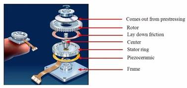
Figure 1. Exploded view of an annular travelling wave motor

§ The rotor: It can be separated in 3 zones:

§ The axis, output of the motor;

§ The track friction in contact with the stator;

§ The spring fold linking axis to track and giving the elasticity needed to apply rotor on stator.

Stator/rotor interface: The model of the interface stator-rotor is the most complex part in the ultrasonic motor model. It is supposed that the stator is rigid and its vibration profile does not change after the contact with the rotor, knowing that this one has a conform layer of contact. This part is the one where the interne functional behaviour is assured by the existence of some forces. These forces depend on comparison between the displacements speeds of the stator and the rotor respectively [9].

One of manners to describe the mechanics of contact is to employ the model of contact zone showed in Figure 2. This model supposes that the stator is rigid and the rotor has a contact layer specified as a linear spring with an equivalent rigidity in the axial and tangential direction.

Electric equivalent circuit

Depicted in Figure 3, r_L is a function of the load torque and applied pre-load pressure. This resistor will model the vibration taking place during the actuation of the motor. It will also take into account of the mechanical and viscous losses in the bearing and other related parts of the ultrasonic motor [3]. Due to the complexity of the interaction between the stator and the rotor, the value of r_L has yet to be established. In our case, it will be derived experimentally to establish their relationship.

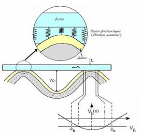
Figure 2. Overlapping between the stator surface and the contact layer of the rotor

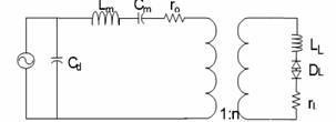
Figure 3. Single phase equivalent circuit for motor

The blocking capacitance C_d lowers the power factor. It would have no effect on the motor’s efficiency if there were no line resistance connected between the power supply and the motor. However, under actual operating condition, a lower power factor adversely affects the efficiency, owing to the power source’s high internal resistance. To improve the power factor, we can place an inductor in parallel to C_d as shown in Figure 4.

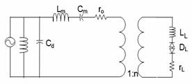
Figure 4. Canceling the effect of blocking capacitance

If C_d is completely cancelled by the inductor, we can then use the simplified equivalent circuit in Figure 5.

Although one may find the physical significance and relationship of the electrical elements in the equivalent circuit easy to understand, its computational analysis is tedious because the diode is a non-linear element [6].

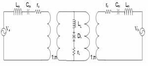
Figure 5. Electric equivalent circuit for the complete motor

As the objective of this research is to find a fast and accurate method to predict the performance of RUSM, we will introduce a few approximations to construct a simplified equivalent circuit in order to keep the computations at a manageable level. For the individual phase A and B, the losses and outputs are quantities that vary sinusoidally. Even though the phase difference between A and B is 90, the losses or output power is in fact 180 as they are expressed in terms of the squares of either the current or the voltage. If these quantities are added together, the resultant is a constant. Since the friction is the predominant driving force and the mass of the rotor is insignificant compared to the pre-load force, we will ignore the effect of LL. If we separate the equivalent circuit for phases A and B by removing the diode and the inductor, with the resistor representing all mechanical losses, we can treat the circuit as a simple A.C. circuit.

Model Compilation and Validation

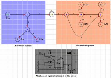
Figure 6. Model Bond Graph of stator with one excitation

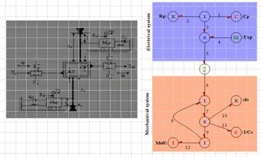
Figure 7. Model Bond Graph for the complete motor

After the exhibition of the used graphical model, with Bond Graph approaches, our task is to implement this model on SYMBOLS; we have implanted the uncoupled Bond Graph model.

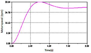
Figure 8. The motor speed without load

The Figure 8 represents the motor speed without load. The figures 9 and 11 show the evolution of the rotation speed as a function of different loads applied.

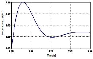
Figure 9. Motor speed as a function of time for a load of 2N

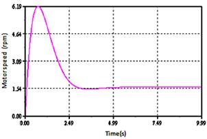
Figure 10. Motor speed as a function of time for a load of 3N

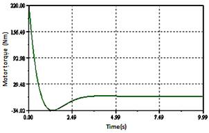
Figure 11. Evolution of traction force a function of time for a load of 300N

Considering the parameter values of the motor used for the simulation (see Table 1), the Bond Graph model developed was simulated, in the steady and transient state of motor. The optimal parameters of the excitation voltages frequency have been tracked and evaluated to 46.65 kHz as frequency, 570 volt as excitation voltages amplitude and π/2 rd as the shift between the two excitations.

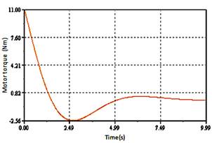
Figure 12. Evolution of traction force a function of time for a load of 3N

The performances of the motor were estimated by applying various loads in the phase of the steady state after 1.5s of operation. The influence of the application of the loads and consequently the evolution of torque and rotor speed are presented in the following figures.

The figure 8 represents the rotor speed without load. The figures 9 and 10 described revolving rotor speed for different cases loads. From times 1.5 second, the motor was loaded by load torque of 2Nm, 3Nm, 300Nm. It will be noticed that the speed decreases, when the applied load increases.

The figures 11 and 12 shows the motor torque characteristics for various loads, which illustrate what happens if a load torque is applied to the rotor after 2s of operation: the driving torque provided by the stator has to increase in order to balance the load torque. Therefore, the driving zone widens (the no-slip points move away from the wave crests), whereas the braking zones contract. The rotor velocity is equal to the stator horizontal velocity at the no slip points; therefore, moving no slip points down the velocity profile cause the rotor to slow down.

Table1. Parameters of motor

Name	Symbol and value
Resistances of entries	Rp=5 - Ds=5
Ceramics capacity	Cp=7.8E-9 F - 1/Cs=7.87E-9 F
Capacity of stator	CM=0.42E-9 - Cp= 0.428E-9
Effective mass	Meff = 40.5 Kg
Mass of rotor	LM=(meff+22.8+3)*1e-3 Kg
The distance enters the points of surface of stator	a=4.5E-3 m
Frequency of Resonance	Wres2=wres1 - wres1=2*pi*43.365*1E+3 Hz
Wavelength	λ=2*pi*R w/n m

Fault Detection and Isolation (FDI)

A number of methods have been developed for fault detection and isolation. All methods of fault detection work by designing residual functions. The residual represents the difference between an estimated value and a measured one, which should be zero during normal operation, but large in the presence of faults [10].

In practice, there is a distinction between the detection of fast-acting, possibly safety-critical faults, and faults which are non-safety-critical and slower to develop, for example due to wear. The former are most likely to be detected by state-estimation and instantaneous comparison of prediction with measurement, while the latter are detected using parameter estimation techniques which require a certain time window and excitation of the system.

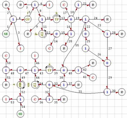
Figure 13. Bond Graph model

Probability analysis can be used to judge, from the residual values, when a fault or change has taken place. This paper is concerned primarily with detection of fast-acting faults, detected via state estimation.

Isolation, in the literature, means diagnosis of the faulty component. If faults are allowed to occur simultaneously, then for a diagnosis, at least as many independent residual functions as faults considered are required. In practice, it is usually assumed that only one fault occurs at a time, which facilitates more robust fault diagnosis [7]. The Bond Graph model of the process is represented by Figure 2.

Analytical Redundancy Relations

Analytical Redundancy Relations (ARR) are symbolic equations representing constraints between different known process variables (parameters, measurements and sources). ARR are obtained from the behavioural model of the system through different procedures of elimination of unknown variables.

Numeric evaluation of each ARR is called a residual, which is used in model based Fault Detection and Isolation (FDI) algorithms.

Technical Specifications for Sensors Placement

The goal of these sections is to provide an optimal sensor placement method on the Bond Graph model in order to make all components monitorable.

We assume that the faults are not multiple and may affect only components. Let given a Bond Graph model obtained from physical process. We suppose that the sensors are not placed yet on the Bond Graph model [10].

Let x_i and y_j the Boolean variables to express the potential sensor placement on the junction nodes such as:

Let:

· N₀ number of “0” junctions

· N₁number of “1” junctions

· n_i number of bonds around the i^th  “0” junction (i = 1, N0)

· m_j number of bonds around the j^th “1” junction (j = 1, N1)

· In the following, “f”and “e” denote flow and effort vector, respectively.

Equations of the i^th “0” junction are:

Equations of the j^th “1” junction are:

For the “0” and the “1” junction, the unknown variable (based on fixed causality) is calculated as flows:

(1)

where s denotes the Laplace variable for a linear system.

(2)

For our application, the equations in junctions are given by:

For 1_{i(i=0, 16)} junction:

(3)

For 0_{j(j=1, 6)} junction:

(4)

From equations of junctions we generate the following Analytical Redundancy Relation:

(5)

From the binary variables x_i and y_j we can determine the final structure of the monitorable system [2]. Two 10-sensor placement combinations provide the monitorability of the all components. The question arises whether we are able to supervise this system by only 9 sensors? And what are the combinations which provide this result?

The signature for [y₁y₂y₃y₄y₅y₆y₇y₈x₁x₂]=[0111111111] is presented in Table 2.

Table 2. Table signature for [y₁y₂y₃y₄y₅y₆y₇y₈x₁x₂]=[0111111111]

	I1	I2	R4	R5	R6	r2	I3	I4	C1	C2
ARR1	1	1	0	0	0	0	0	0	0	0
ARR2	0	0	1	0	0	0	0	0	0	0
ARR3	0	0	0	1	0	0	0	0	0	1
ARR4	0	0	0	0	1	0	0	0	0	1
ARR5	0	0	0	0	0	1	0	0	0	1
ARR6	0	0	0	0	0	0	1	0	0	0
ARR7	0	0	0	0	0	0	0	1	0	0
ARR8	0	0	0	0	0	0	0	0	1	0
ARR9	0	0	0	0	0	0	0	0	0	1

The fault signatures are not different from each other (I₁ and I₂) and not equal to zero, then the components I₁ and I₂ are not monitorable but R₄, R₅, R₆, r₂, I₃, I₄, C₁ and C₂ are monitorable.

The signature for [y₁y₂y₃y₄y₅y₆y₇y₈x₁x₂]=[1111111110] is presented in Table 3.

The fault signatures are different from each other and not equal to zero, then the components I₁, I₂, R₄, R₅, R6, r₂, I₃, I₄, C₁ and C₂ are monitorable.

Table 3. Table signature For [y₁y₂y₃y₄y₅y₆y₇y₈x₁x₂]=[1111111110]

	I1	I2	R4	R5	R6	r2	I3	I4	C1	C2
ARR1	1	0	0	0	0	0	0	0	0	0
ARR2	0	1	0	0	0	0	0	0	0	0
ARR3	0	0	1	0	0	0	0	0	0	1
ARR4	0	0	0	1	0	0	0	0	0	1
ARR5	0	0	0	0	1	0	0	0	0	1
ARR6	0	0	0	0	0	1	0	0	0	0
ARR7	0	0	0	0	0	0	1	0	0	0
ARR8	0	0	0	0	0	0	0	1	0	0
ARR9	0	0	0	0	0	0	0	0	1	0

Simulation and Interpretation

From SYMBOLS 2000, we have implanted the uncoupled Bond Graph model.

For the faults detection of ultrasonic linear motor we use the precedent Analytical Redundancy Relations (ARRs). We create the faults on monitoring components with this software fault here is considered in the total absence or the deviation of the nominal value given out by the component to monitor.

The numeric values of components are not considered, only their presence or absences in the relation are taken in account with evaluation term the operators (+, -). It is the qualitative approach for Bond Graph monitoring.

Monitoring of I₁ and the resistance R₁

In the first time, we create a fault between the instant t = 2 and t = 2.5 s .The diagram bloc of process is presented in Figure 14 while sensitivity of detector Df₁ is presented in Figure 15.

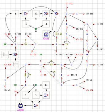
Figure 14. Diagram bloc

The failures on I₁ and R₁ are characterized by the presence of the detector Df₁ in the analytical redundancy relation ARR₁. We note that the residual ARR₁ is sensitive to the failures which affect I₁ and R₁, but residuals ARR₂, ARR₃, ARR₄, ARR₅, ARR₆, ARR₇, ARR₈ and ARR₉ are equals to zero.

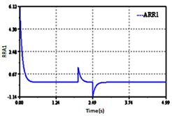
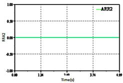
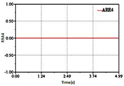
Figure 15. Sensitivity of detector Df₁

Monitoring of I₂ and the resistance R₂

By the same procedure we can monitored the components I₂ and R₂.

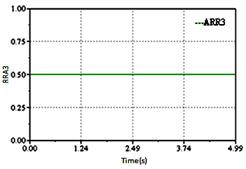
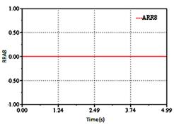
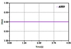
Figure 16. Sensitivity of detector Df₂

The generated ARRs reaction is very fast see Figure 16. The deviation of the relations ARR₁, ARR₄, ARR₅, ARR6, ARR₇, ARR₈ and ARR₉ in this time is normal (constant value).

We see that residuals ARR₂ is sensitive (seen the presence of Df₂ in this relation).

Monitoring of C₁

The deviation of the relations ARR₁, ARR₂, ARR₃, ARR₄, ARR₅, ARR₆, ARR₇ and ARR₈ in this time is normal (constant value). We see that residual ARR₉ are sensitive (seen the presence of De₁ in this relation, Figure 17).

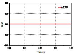
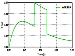
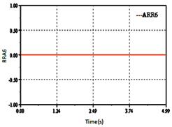
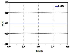
Figure 17. Sensitivity of detector De1

Results and Discussions

This work has presented piezomotor and more precisely, travelling wave ultrasonic annular motor. Its advantages and drawback have been explained. Piezomotors have specificities that are very interesting if they match application’s needs: high torque/low speed, holding torque, silent operation, reactivity, high integration level. Because of the ultrasonic linear motor’s complexity, precise analysis using analytic method is very difficult. Nevertheless, this modeling methodology has been presented in order to show that it is possible to model ultrasonic motors analytically. In the same way, the method of Bond Graph could be applied. Bond Graph is an explicit graphical tool for capturing the common energy structure of systems. In the vector form, it gives a concise description of complex systems. By this approach, a physical system can be represented by symbols and lines, identifying the power flow paths.

The method used illustrates the process principle working. We have using the structural junction equations for generating the analytical redundancy relations like failures indicators. The Bond Graph tool is the unified modelling method and it facilitates the functional and structural analysis of the complex systems. The multi-energy Bond Graph based approach used here for fault detection of the complex systems will be in perspective following by fault isolation and identification of eventual failure.

The tool Bond Graph and software SYMBOLS 2000 are proven powerful and convenient means for this project which included the modelling, the monitoring, the simulation and the analysis of the results. The results found here are proven interesting because the simulation of defects in quite precise moments were confirmed by the software of simulation starting from the sensitivity of the indicators installed.

Conclusion

The main contribution of the work presented in this paper consists in the description of Bond Graph modelling of travelling wave ultrasonic motor, and simulation characteristics.    The modelling of the travelling wave ultrasonic motor and its simulation is an important task to understand the principle of operation and its dynamic behaviour.

The generation of the analytical redundancy relations by the Bond Graph approach shows some interesting characteristics:

§ They are simple to include/understand, since they correspond to relations and variables which are posted by the model Bond Graph image of the physical process, these relations are deduced directly from the graphic representation.

§ They can be generated in form symbolic system and thus adapted to a data-processing implementation.

References

1. Jaume D., Verge M., Modélisation structurée des systèmes avec les Bond Graph, Edition Technip, 2004.

2. Pifort V., Preumont A., Finite element modeling of piezoelectric structures, Active Structures Laboratory ULB, 2001.

3. Fukunaga H., Kakehashi H., Ogasawara H., Ohta Y., Effect of Dimension on Characteristics of Rosen-Type Piezoelectric Transformer, IEEE International Ultrasonics Symposium, 1998.

4. Hagood N.W., Andrew J., Modeling of a Piezoelectric Rotary Ultrasonic Motor, IEEE Transactions on Ultrasonic, Ferroelectrics, and Frequency Control, 1995, 42(2), p. 210-224.

5. Jeong S.H., Lee H.K., Kim Y.J., Kim H.H., Lim K.J., Vibration analysis of the stator in ultrasonic motor by FEM, Proceedings of the 5th International Conference on Properties and Applications of Dielectric Materials, 1997, pp. 1091-1094.

6. Kawamura A., Takeda N., Linear Ultrasonic Piezoelectric Actuator, IEEE Trans. on Industry Applications, 1991, 27(1), p. 23-26.

7. Samantaray A.K., Medjaher K., Ould Bouamama B., Staroswiecki M., Dauphin-Tanguy G., Diagnostic bond graphs for online fault detection and isolation, Simulation Modeling Practice and Theory Journal, 2005, p. 237-262.

8. Borutzky W., Bond Graphs a Methodology for Modeling Multidisciplinary Dynamic Systems, volume FS-14 of Frontiers in Simulation, SCS Publishing House, Erlangen, San Diego, 2004.

9. Helin P., Sadaune V., Druon C., Tritch J. B., A Mechanical Model for Energy Transfer in Linear Ultrasonic Micromotors Using Lamb and Rayleigh Waves, IEEE/ASME Transactions on Mechatronics, 1998, 3(1), p. 3-8.

10. Khemliche M., Ould Bouamama B., Haffaf H., Sensors placement for diagnosability on Bond Graph model, Sensors and Actuators Journal, 2006, 4, p. 92-98.