A Hybrid Approach for Automatic Classification of Brain MRI Using Genetic Algorithm and Support Vector Machine

Ahmed KHARRAT^1,*, Karim GASMI¹, Mohamed BEN MESSAOUD², Nacéra BENAMRANE³ and Mohamed ABID¹

¹Computer & Embedded Systems Laboratory (CES)

²Laboratory of Electronics and Information Technologies, National Engineering School of Sfax, BP 1173-3038 Sfax, Tunisia

³ Vision and Medical Imagery Laboratory, Department of Computer Science Faculty of Science, U.S.T.O., B.P 1505, EL-Mnaouer, Oran, 31000, Algeria

E-mails: Ahmed.Kharrat@ieee.org, gasmikarim@yahoo.fr, M.BenMessaoud@enis.rnu.tn, nabenamrane@yahoo.com, Mohamed.Abid@enis.rnu.tn

^* Corresponding author E-mail: Ahmed.Kharrat@ieee.org

Received: 21 August 2010 / Accepted: 29 December 2010 / Published: 30 December 2010

Abstract

We purpose a hybrid approach for classification of brain tissues in magnetic resonance images (MRI) based on genetic algorithm (GA) and support vector machine (SVM). A wavelet based texture feature set is derived. The optimal texture features are extracted from normal and tumor regions by using spatial gray level dependence method (SGLDM). These features are given as input to the SVM classifier. The choice of features, which constitute a big problem in classification techniques, is solved by using GA. These optimal features are used to classify the brain tissues into normal, benign or malignant tumor. The performance of the algorithm is evaluated on a series of brain tumor images.

Keywords

Support vector machine; Genetic algorithm; Spatial grey level dependence method; Texture features; Wavelet transform

Introduction

Brain tumor is any mass that results from abnormal growths of cells in the brain. It may affect any person at almost any age. Brain tumor effects may not be the same for each person, and they may even change from one treatment session to the next. Brain tumors can have a variety of shapes and sizes; it can appear at any location and in different image intensities. Brain tumors can be benign or malignant. Low grade Gliomas and Meningiomas [1], which are benign tumors, represent the most common type of brain tumor. Glioblastoma multiform [1] is a malignant tumor and represents the most common primary brain neoplasm. Benign brain tumors have a homogeneous structure and do not contain cancer cells. They may be either simply be monitored radiologically or surgically eradicated and they seldom grow back. Malignant brain tumors have a heterogeneous structure and contain cancer cells. They can be treated by radiotherapy, cheomotherapy or a combination thereof and they are life threatening. Many procedure and diagnostic imaging techniques can be performed for the early detection of any abnormal changes in tissues and organs such as Computed Tomography (CT) scan and Magnetic Resonance Imaging (MRI) [2]. Although MRI seems to be efficient in supplying the location and size of tumors, it is unable to classify tumor types, hence the application of biopsy [2]. Biopsy is a painful process. This inability requires development of new analysis techniques that aim at improving diagnostic ability of MR images.

Many techniques have been reported for classification of brain tumors in MR images, most notably, support vector machine (SVM) [3] neural network [4], knowledge based techniques [5], expectation–maximization (EM) algorithms and Fuzzy c-means (FCM) clustering. An SVM is a machine learning system developed using statistical learning theories to classify data points into two classes. Notably, SVM models have been applied extensively for classification, image recognition and bioinformatics. Chang et al. [6, 7] show the SVM is an effective tool in sonography for the diagnosis of breast cancer. In the same context, Luiza Antonie [8] proposed a method for Automated Segmentation and Classification of Brain MR images in which an SVM classifier was used for normal and abnormal images classification with statistical features. Chaplot et al [9] observed that the classification rate is higher for a support vector machine classifier than neural networks self-organizing maps-based approach. SVMs are suggested to show their superior performance and feasibility in the classification of brain tissues in classical maximum-likelihood methods. Gering et al. [10] applied the EM algorithms in the detection of abnormalities. These algorithms proved to be capable of distinguishing large tumors from the surrounding brain tissues by training exclusively on normal brain images in healthy people in order to recognize deviation from normality. This requires high computational effort. The knowledge based techniques allowed to make more efficient segmentation and classification results but these techniques required intensive training.

In medical image analysis, the determination of tissue type (normal or pathological) and classification of tissue pathology are performed by using texture. MR image texture proved to be useful to determine the tumor type [11] and to detect Alzheimer’s disease [12].

To solve the texture classification problem many approaches have been developed over the years, such as multichannel methods, multi-resolution analysis, level set, Gabor filters, and wavelet transform [13, 14]. Gabor filters are poor due to their lack of orthogonality that results in redundant features at different scales or channels. While Wavelet Transform is capable of representing textures at the most suitable scale, by varying the spatial resolution and there is also a wide range of choices for the wavelet function.

There is a big problem in selecting the optimal features to distinguish between classes. The evaluation of possible feature subsets is usually a painful task due to the large amount of computational effort required. Genetic algorithms (GAs) appear to be a seductive approach to choose the best feature subset while maintaining acceptable classification accuracy. Siedlecki and Sklansky [15] compared the GA with classical algorithms and they concluded the superiority of the GA.

A new method for extracting features in MR images with lower computational requirements are proposed, and classification results are analyzed.

Material and Method

Proposed image analysis process is outlined in Figure 1.

Figure 1. The Image Analysis process

For feature extraction we use the method proposed by Haralick [16], namely, the spatial gray-level dependence method (SGLDM). This well known statistical method for extracting second order texture information is based on the estimation of the discrete second order probability function C(I,J/Δx,Δy,) [16]. This function represents the probability of going from gray level i to gray level j, given that the spacing is d and the direction is given by the angle q. This is also referred to as co-occurrence matrix. For an offset distance d=1, co-occurrence matrices are calculated for offset angles of 0° (in the horizontal direction), 45° (along the positive diagonal), 90° (in the vertical direction), and 135° (along the negative diagonal). In table 1, thirteen Haralick features are described and added with nine features to facilitate our task and to make it more efficient and consistent [16-18]. The mean and range of each measure over the four offset angles are used as features; this yields 44 features.

Table 1. Extracted texture features

Feature number	Feature (mean, range)	Feature number	Feature (mean, range)
1, 2	Angular second moment	23, 24	information measure of correlation I
3, 4	Contrast	25, 26	information measure of correlation II
5, 6	Correlation	27, 28	maximal correlation coefficient
7, 8	Variance	29, 30	Correlation mat
9, 10	inverse difference moment	31, 32	Cluster Prominence
11, 12	sum average	33, 34	Cluster Shade
13, 14	sum variance	35, 36	Dissimilarity
15, 16	sum entropy	37, 38	Energy
17, 18	Entropy	39, 40	Homogeneity
19, 20	difference variance	41, 42	Maximum probability
21, 22	difference entropy	43, 44	Inverse difference normalized

In the proposed method, we perform a second level decomposition of image. These images are decomposed using 2D wavelet transform into four subbands. The wavelet transform is Daubechies wavelet filter of order two, level 1 [19]. The subband with low frequency represents the clearest appearance of the changes between the different textures. The later are extracted from the subband which has maximum variance and low frequency.

Feature Selection and Optimization using GA

In a classification problem, the number of features can be quite large, many of them can be irrelevant or redundant. Feature reduction improves classification by searching for the best features subset, from the fixed set of the original features, according to a given processing goal and a feature evaluation criterion: classification accuracy. This is illustrated in Figure 2.

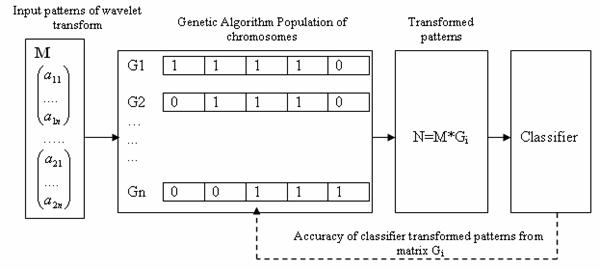
Figure 2. Classification accuracy using a GA-based features extractor

A pattern’s features, from the point of view of processing goal and type, may be irrelevant (having no effect on processing performance) or relevant (having an impact on processing performance) or redundant (correlated, dependent). Hence to reduce the large number of features to a smaller set of features we apply GA-based global search method. GA is an adaptive method of global-optimization searching and simulates the behavior of the evolution process in nature. It is based on Darwin’s fittest principle, which states that an initial population of individuals evolves through natural selection in such a way that the fittest individuals have a higher chance of survival [20]. The GA maintains a population of competing feature transformation matrices. To evaluate each matrix in this population, the input patterns are multiplied by the matrix, producing a set of transformed patterns which are then sent to a classifier. The classifier typically divides the patterns into a training set, used to train the classifier, and a testing set, used to evaluate classification accuracy. The accuracy obtained is then returned to the GA as a measure of the quality of the transformation matrix used to obtain the set of transformed patterns. Using this information, the GA searches a transformation that minimizes the dimensionality of the transformed patterns and maximizing classification accuracy. Each feature is encoded into a vector called a chromosome. One element of the vector represents a gene. Each bit in the binary vector is associated with a feature. If the i^th bit of this vector is equal to one then the i^th feature is allowed to participate in classification. All of the chromosomes make up of a population and are estimated according to the fitness function in the equation (1).

fitness = WA∙Accuracy + Wnb/N

(1)

where W_A is the weight of accuracy and W_nb is the weight of N feature participated in classification where N ≠ 0.

A fitness value will be used to measure the fitness of a chromosome and decides whether a chromosome is good or not in a population. Initial populations in the genetic process are randomly created. GA uses then three operators to produce a next generation from the current generation: reproduction, crossover and mutation. GA eliminates the chromosomes of low fitness and keeps the ones of high fitness.

Thus more chromosomes of high fitness move to the next generation. This process is repeated until a good chromosome (individual) is found. The figure 3 illustrates the feature selection using the genetic algorithm.

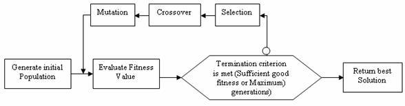
Figure 3. Feature Selection using GA

Classification using SVM

Support Vector Machine (SVM) is a powerful supervised classifier and accurate learning technique that has been introduced in 1995. It is derived from the statistical theory developed by Vapnick in 1982 [21]. It yields successful classification results in various application domains, e.g. medical diagnosis [22, 23]. Support Vector Machine (SVM) is based on the structural risk minimization principle from the statistical learning theory. Its kernel is to control the empirical risk and classification capacity in order to maximize the margin between the classes and minimize the true costs [24]. A support vector machine searchs an optimal separating hyper-plane between members and non-members of a given class in a high dimension feature space [25]. The inputs to the SVM algorithm are the feature subset selected using GA during data pre-processing step and extracted using the SGLDM method. In our method, the two classes are normal or abnormal brain. Then classification procedure continues to divide the abnormal brain into malignant and benign tumors; each subject is represented by a vector in all images. There are many common kernel functions, such as:

• Linear: x_i·x_j,
• Polynomial of degree d: (x_i·x_j + 1)^d,
• Radial basis function (RBF): .

Among these kernel functions, a radial basis function proves to be useful, due to the fact the vectors are nonlinearly mapped to a very high dimension feature space. The optimal values of constants γ and C are determined, where γ is the width of the kernel function and C is the error/trade-off parameter that adjusts the importance of the separation error in the creation of the separation surface. We perform the classification for the MRI dataset with (γ, C) varying along a grid. SVM-based classification takes N training samples, trains the classifier on N-1 samples, then uses the remaining one sample to test. This procedure is repeated until all N samples have been used as the test sample. The performance of the classification for a given value (γ, C) is evaluated by computing the accuracy across all subjects.

Results and Discussion

Our proposed hybrid techniques are implemented on a real human brain dataset. The input dataset consist in 83 images: 29 images are normal, 22 malignant tumors suffering from a low grade Glioma, Meningioma and 32 benign tumors suffering from a Bronchogenic Carcinoma, Glioblastoma multiform, Sarcoma and Grade IV tumors. These normal and pathological benchmark images used for classification, are axial, T2-weighted of 256´256 sizes and acquired at several positions of the transaxial planes. These images were collected from the Harvard Medical School website [26]. We have considered that all images belonging to seven persons (four men and three women). Their ages vary between 22 and 81 years. The determination of MR tumor type, which can be achieved by the histopathological analysis of biopsies, was considered as the gold standard for the classification of images. A typical representative MR image of normal, benign and malignant tumor is shown in Figure 4.

Once our data set is collected, we follow different steps of our system described in the previous Sections. For the extraction step we apply SGLDM to extract 13 features. Additional 9 features are also extracted for the performance of our method. This yields a total of 44 features including the mean and the range.

(a) normal brain

(b) benign tumor

(c) malignant tumor

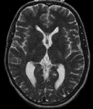
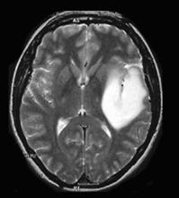
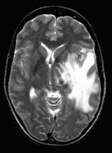
Figure 4. Three T2 weighted MR images in axial plane

Due to the small size of the dataset, the SVM classifier is employed. In the classification step we choose the RBF kernel due to the fact that many studies have demonstrated that the preferable choice is RBF [27], and the technique used to fix its optimal parameters is a grid search using a cross-validation. Cross-validation method with 5 folders is used to search the best parameters among an interval of values which achieve a high accuracy during training and testing phases. Hence, the values of C and γ are 8 and 2, respectively as the best parameters to apply in our implementation. Having as input these 44 extracted features, GA is performed to reduce the number of features. The feature set containing five features is used as entries of SVM classification. These optimal features mean of contrast, mean of homogeneity, mean of sum average, mean of sum variance and range of autocorrelation [28]. A population of 30 chromosomes is randomly generated. Each chromosome contains 44 genes (One gene for each feature). The genetic operators, one point crossover and mutation are used. The crossover rate is 90% and mutation rate is 10%. Tournoi selection method is used to select the mating pool.

In this section, we present the performance evaluation methods used to evaluate the proposed approaches. We assess the performance of the proposed method in terms of sensitivity, specificity and accuracy. The three terms are defined in Equations (2)-(4):

Sensitivity=TP/(TP+FN) 100%	(2)
Specificity = TN/(TN+FN) 100%	(3)
Accuracy = (TP+TN)/(TP+TN+FP+FN) 100%	(4)

where:

TP (True Positives) = correctly classified positive cases,

TN (True Negative) = correctly classified negative cases,

FP (False Positives) = incorrectly classified negative cases,

FN (False Negative) = incorrectly classified positive cases.

Sensitivity (true positive fraction) is the probability that a diagnostic test is positive, given that the person has the disease. Specificity (true negative fraction) is the probability that a diagnostic test is negative, given that the person does not have the disease. Accuracy is the probability that a diagnostic test is correctly performed.

Table 2 shows the classification rates for performing the proposed hybrid approach by using the most common kernel functions including linear, polynomial of degree and RBF.

Table 2. Classification results from support vector machine

Kernel used	Total № of images	Number of images						Images misclassified	Classification Accuracy ±SD (%)
		Training			Testing
		Normal	Benign	Malign	Normal	Benign	Malign
Lin	83	12	9	16	29	18	36	3±1	96.36±1.23
Poly	83	12	9	16	29	18	36	2±1	97.59±1.2
RBF	83	12	9	16	29	18	36	2±1	97.59±1.2
Legend: Lin - Linear; Poly - Polynomial; RBF - Radial basis function

In fact classification accuracy varies from 96.36±1.23 to 97.59±1.2 %, with polynomial and radial basis function. Both tools could achieve satisfactory classification results for brain tumor but we prefer the application of RBF. In this case, the classification accuracy varies from 96.39 to 98.79 % in the mean standard deviation format (Mean±SD) of 97.59±1.2 %.

Our hybrid approach is performed to classify the benign or malignant tumor. To evaluate the effectiveness of our method we compare our results with another procedure for the same MRI datasets. The compared approach omits the decomposition step (WT). Table 3 gives the classification accuracies of this approach and our hybrid method composed of four steps.

Table 3. Classification rates (in %) for the proposed technique and the other procedure that lacks the decomposition stage

The hybrid technique	TP	TN	FP	FN	Sensitivity ± SD	Specificity	Accuracy ± SD
SGLDM+GA+SVM	34±1	17	0	3±1	91.87±2.69	100	94.44±1.85
WT+SGLDM+GA+SVM	35±1	17	0	2±1	94.6±2.7	100	96.29±1.85

This comparison shows that our system has high classification accuracy and less computation due to the feature extraction based on WT. In fact, the experimental results show that the accuracy rate in our hybrid approach varies from 94.44 to 98.14 % while in the other approach varies from 92.59 to 96.29 %. Hence the results of classification of proposed approach are better than the other one lacking the decomposition stage for classification of the human brain, benign or malignant tumor. Moreover in our proposal, the sensitivity rate varies from 91.9 to 97.3 % with the mean SD of 94.62.7 %. This makes our approach an efficient clinical image analysis tool for doctors or radiologists to classify MRI tumor and to further obtain MRI tumor location and Vol. estimation.

Conclusions

The paper developed a hybrid technique with normal and benign or malignant classes. Our medical decision making system is designed by the wavelet transform (WT), genetic algorithm (GA) and supervised learning methods (SVM). The proposed approach gives very promising results in classifying the healthy and pathological brain. The benefit of the system is to assist the physician to make the final decision. The proposed algorithm is efficient for classification of the human brain normal or abnormal (benign and malignant tumor) with high sensitivity, specificity and accuracy rates. The performance of this study appears some advantages of this technique: it is accurate, robust easy to operate, non-invasive and inexpensive. The approach is limited by the fact that it necessitates fresh training each time whenever there is a change in image database.

Acknowledgements

The authors would like to thank Dr. Khalil Chtourou, Biophysics and Nuclear Medicine from the CHU Habib Bourguiba, Department of Nuclear Medicine, Tunisia-Sfax, is acknowledged for providing several clarifications on the medical aspects of the datasets.

They also like to be grateful Mrs Ines Kallel for her helpful review of the manuscript.

References

1. Ricci P.E., Dungan D. H., Imaging of low- and intermediate-grade gliomas, Seminars in Radiation Oncology, 2001, 11(2), p. 103-112.

2. Armstrong T.S., Cohen M.Z., Weinbrg J., Gilbert M.R. Imaging techniques in neuro oncology. In Seminars in Oncology Nursing, 2004, 20(4), p. 231-239.

3. Shubhangi D.C., Hiremath P.S., Support vector machine (SVM) classifier for brain tumor detection. International Conference on Advances in Computing, Communication and Control, 2009, p. 444-448.

4. Reddick W.E., Glass J.O., Cook E.N., Elkin T.D., Deaton R.J., Automated segmentation and classification of multispectral magnetic resonance images of brain using artificial neural networks, IEEE Transactions on Medical Imaging, 1997, 16(6), p. 911-918.

5. Clark M.C., Hall L.O., Goldgof D.B., Velthuizen R., Murtagh F.R. and Silbiger M.S., Automatic tumor segmentation using knowledge based techniques, IEEE Transactions on Medical Imaging, 1998, 17(2), p. 187-192.

6. Chang R.F., Wu W.J., Moon W.K., Chou Y.H., Chen D.R., Support vector machines for diagnosis of breast tumors on US images. Academic Radiology, 2003, 10(2), p. 189-197.

7. Chang R.F., Wu W.J., Moon W.K., Chou Y.H., Chen D.R., Improvement in breast tumor discrimination by support vector machines and speckle-emphasis texture analysis, Ultrasound in Medicine and Biology, 2003, 29(5), p. 679-686.

8. Antonie L., Automated Segmentation and Classification of Brain Magnetic Resonance Imaging, C615 Project, 2008, http://en.scientificcommons.org/42455248.

9. Chaplot S., Patnaik L.M., Jagannathan N.R., Classification of magnetic resonance brain images using wavelets as input to support vector machine and neural network, Biomedical Signal Processing and Control, 2006, 1(1), p. 86-92.

10. Gering D.T., Eric W., Grimson L., Kikins R., Recognizing deviations from normalcy for brain tumor segmentation, Lecture Notes in Computer Science, 2002, 2488, p. 388-395.

11. Schad L.R., Bluml S., Zuna, I., MR tissue characterization of intracranial tumors by means of texture analysis, Magnetic Resonance Imaging, 1993, 11(6), p. 889-896.

12. Freeborough P.A., Fox N.C., MR image texture analysis applied to the diagnosis and tracking of Alzheimer’s disease, IEEE Transactions on Medical Imaging, 1998, 17(3), p. 475-479.

13. Dunn C., Higgins W.E., Optimal Gabor filters for texture segmentation, IEEE Transactions on Image Processing, 1995, 4(7), p. 947-964.

14. Chang T., Kuo C., Texture Analysis and classification with tree structured wavelet transform, IEEE Transactions on Image Processing, 1993, 2(4), p. 429-441.

15. Siedlecki W., Sklanky J., A note on genetic algorithms for large-scale feature selection, Pattern Recognition Letters, 1989, 10(5), p. 335-347.

16. Haralick R. M., Shanmugam K., Dinstein I., Textural Features for Image Classification, IEEE Trans On Systems Man and Cybernetics, 1973, 3(6), p. 610-621.

17. Soh L., Tsatsoulis C., Texture Analysis of SAR Sea Ice Imagery Using Gray Level Co-Occurrence Matrices, IEEE Transactions on Geoscience and Remote Sensing, 1999, 37(2), p. 780-793.

18. Clausi D.A., An analysis of co-occurrence texture statistics as a function of grey level quantization, Canadian Journal of Remote Sensing, 2002, 28(1), p. 45-62.

19. Kharrat A., Ben Messaoud M., Benamrane N., Abid M., Detection of Brain Tumor in Medical Images, IEEE 3rd International Conference on Signals, Circuits & Systems, 2009, 6p, DOI: 10.1109/ICSCS.2009.5412577.

20. Goldberg D.E., Genetic Algorithms in search, Optimization and Machine Learning, Boston, MA, USA, Addison-Wesley Longman, 1989.

21. Vapnik V.N., Estimation of Dependences Based on Empirical data, Secaucus, NJ, USA, Springer-Verlag New York, 1982.

22. Guyon I., Weston J., Barnhill S., Vapnik V., Gene Selection for Cancer Classification using Support Vector Machines, Machine Learning, 2002, 46(1-3), p. 389-422.

23. Zhang J., Liu Y., Cervical Cancer Detection Using SVM Based Feature Screening, Proc of the 7th Medical Image Computing and Computer-Assisted Intervention, 2004, 2, p.873-880.

24. Zhang K., CAO H.X., Yan H., Application of support vector machines on network abnormal intrusion detection. Application Research of Computers, 2006, 5, p.98-100.

25. Kim D., Park J., Network-based intrusion detection with support vector machines, Lecture Notes in Computer Science, 2003, 2662, p. 747-756.

26. Harvard Medical School, http://med.harvard.edu/AANLIB/

27. Scholkopf B., Smola A.J., Learning with Kernels Support Vector Machines, Regularization, Optimization and Beyond, Cambridge, MIT Press, 2001.

28. Kharrat A., Gasmi K., Ben Messaoud M., Benamrane N. and Abid M., Automated Classification of Magnetic Resonance Brain Images Using Wavelet Genetic Algorithm and Support Vector Machine. The 9th IEEE International Conference on Cognitive (ICCI 2010), July 7-9, 2010, Tsinghua University, Beijing, China. (Accepted for publication).