Optimal Reactive Power Dispatch Considering FACTS Devices
Ismail MAROUANI*, Tawfik GUESMI, Hsan HADJ ABDALLAH and Abdarrazak OUALI
Sfax National Engineering School, Electrical Department. BP W, 3038 Sfax, Tunisia
E-mail: ismail.marouani@isetks.rnu.tn, tawfik.guesmi@istmt.rnu.tn,
hsan.haj@enis.rnu.tn, abderrazak.ouali@enis.rnu.tn
*Corresponding author E-mail: ismail.marouani@isetks.rnu.tn
Received: 29 November 2010 / Accepted: 16 March 2011 / Published: 28 June 2011
Abstract
Because their capability to change the network parameters with a rapid response and enhanced flexibility, flexible AC transmission system (FACTS) devices have taken more attention in power systems operations as improvement of voltage profile and minimizing system losses. In this way, this paper presents a multi-objective evolutionary algorithm (MOEA) to solve optimal reactive power dispatch (ORPD) problem with FACTS devices. This nonlinear multi-objective problem (MOP) consists to minimize simultaneously real power loss in transmission lines and voltage deviation at load buses, by tuning parameters and searching the location of FACTS devices. The constraints of this MOP are divided to equality constraints represented by load flow equations and inequality constraints such as, generation reactive power sources and security limits at load buses. Two types of FACTS devices, static synchronous series compensator (SSSC) and unified power flow controller (UPFC) are considered. A comparative study regarding the effects of an SSSC and an UPFC on voltage deviation and total transmission real losses is carried out. The design problem is tested on a 6-bus system.
Keywords
Multi-objective optimization; Evolutionary algorithms; Power flow; static synchronous series compensator (SSSC); unified power flow controller (UPFC); Voltage profile.
Introduction
The ORPD problem is considered as a MOP. It consists to improve the voltage profile and minimize the real power loss in transmission lines under several equality and inequality constraints. Such as, load flow equations and security limits. To maintain the load buses voltage within their permissible limits many technical methods are proposed [1, 2], such as, reallocating reactive power generation in the system adjusting transformer taps, generator voltage and switchable reactive power sources. To minimize system losses, a redistribution of reactive power in the network can be used [3].
Because the recent progress of power electronics, FACTS devices have taken more attention in transmission power systems. They have the capability to change the network parameters with a rapid response and enhanced flexibility, such as, improving voltage profile and minimizing system losses.
Some types of those devices, are, static synchronous series compensator (SSSC), static synchronous compensator (STATCOM) and unified power flow controller (UPFC).
SSSC is considered as a controllable voltage source inverter that is connected in series with transmission line. This injected voltage is almost in quadrature with the line current. Consequently, it provides a variable reactance in series with the transmission line, which, can be inductive or capacitive. This reactance controls the power flow in the line where it is introduced. The STATCOM is a shunt connected FACTS devices. It consists of a voltage source converter linked to the system via a shunt transformer. Its principal function is to ameliorate the voltage profile at the point of connection. To exploit the benefits of those two devices, the UPFC can be a combination of SSSC and STATCOM.
In a MOP, there isn’t one solution that is best with respect to all objectives. Generally, the aim is to determine the trade-off surface, which is a set of non-dominated solution points, known as Pareto optimal solutions. Every individual of this set is an acceptable solution.
In the literature, several methods are used to solve the ORPD. In [2], a nonlinear programming technique was used. Gradient-based optimization algorithms consist to linearize the objective functions and the system constraints around an operating point was presented in [3]. Those traditional techniques consume an important computing time and they are iterative methods. Also, they can converge to a local optimum.
Recently, genetic algorithms (GA) are very much used to solve MOP. Many researchers have transformed the MOP to a single objective problem using appropriate weights. Then, GA was been applied [4]. Unfortunately, the obtained solution depends on the weight vector used in the process. Also, this method requires a number of runs equal to the size of the desired Pareto optimal solutions.
MOEAs are used to eliminate most difficulties of these methods. MOEAs are no iterative and they give the Pareto optimal solutions in one run. Thus, in this article a no conventional technique based on MOEA is employed. It is based on non-dominated Sorting Genetic Algorithm II (NSGAII) approach. Which is an elitist approach and it can maintain population diversity in the set of the non-dominated solutions.
Therefore, the objective of the present paper is to develop a power flow model for power system with FACTS devices. The modified Newton-Raphson power flow algorithm was used [5]. Then, a new ORPD problem is formulated. The solutions of this problem are the FACTS parameters and location.
Static models of two FACTS devices consisting of UPFC and SSSC have been used in the present work.
Material
As indicated previously, SSSC and UPFC are used and mathematically modelled in this paper.
SSSC Mathematical Modelling
Figure 1 shows the circuit model of an SSSC connected at position d between two buses n and m. So, another two buses i and j are added to the total number of buses of the system.
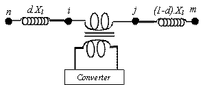
Figure 1. SSSC location between
buses n and m (where d is the portion of the impedance of line n-m,![]() )
)
In its equivalent circuit shown in Figure 2, the SSSC is represented by a voltage source Vse in series with the transformer impedance Xs [6, 7]. In practice, Vse can be regulated to control the power flow of line m-n and the voltage at buses i and j.

Figure 2. Voltage-source model of SSSC
This last model can be developed by replacing voltage source Vse by a current source Ise parallel with the transmission line as shown in Figure 3.

Figure 3. Replacement of series voltage source by a current source
|
Ise = -jbseVse |
(1) |
|
Vse=rViejγ |
(2) |
where r and γ are respectively the p.u. magnitude and phase angle of series voltage source.
0 ≤ r ≤ rmax and 0 ≤ γ ≤ 2π
The power injection model of the SSSC can be seen as two dependent power injections at auxiliary buses i and j as shown in Figure 4 [8].

Figure 4. SSSC mathematical model
The apparent power supplied by the model is calculated as:
|
Si = Vi(-Ise)* |
(3) |
|
Sj = Vj(Ise)* |
(4) |
Then, active and reactive power supplied by the SSSC can be deduced from Equations (5) to (8).
|
Pi,SSSC = -rbseVi2sin(γ) |
(5) |
|
Qi,SSSC = -rbseVi2cos(γ) |
(6) |
|
Pi,SSSC = rbseViVjsin(αi-αj+γ) |
(7) |
|
Qi,SSSC = rbseViVjcos(αi-αj+γ) |
(8) |
UPFC Mathematical Modelling
An UPFC can be represented as shown in Figure 5. It consists of, two voltage sources Vse and Vsh, and two transformer impedances Xse and Xsh. Voltage sources Vse and Vsh are controllable in both their magnitude and phase angles [9, 10].
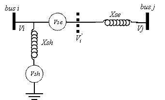
Figure 5. Two voltage-source model of UPFC (where Vse is defined as in Equation (2))
The voltage source Vse in the last model can be replaced by a current source Ise parallel with the transmission line as shown in Figure 3.
The shunt branch in UPFC is employed mainly to provide all the losses in the UPFC and the active power, Pseries, which is injected with the system by the series branch.
If the total losses of the two converters are estimated to be about 2% of Pseries, then, the provided power by shunt branch Pshunt will be expressed by [5]:
|
Pshunt = -1.02Pserie |
(9) |
The function of the reactive power delivered or absorbed by the shunt branch is to maintain the level of tension to bus i within acceptable limits. Finally, UPFC mathematical model can be constructed by combining the series and shunt power injections at both bus i and j as shown in Figure 6 [5].
The elements of equivalent power injection in Figure 6 are:
|
Pi,ufc = 0.02rbseVi2sinγ-1.02rbseViVjsin(αi-αj+γ) |
(10) |
|
Pj,upfc = rbseViVjsin(αi-αj+γ) |
(11) |
|
Qi,upfc = -rbseViVjcos(γ) |
(12) |
|
Qj,upfc = rbseViVjcos(αi-αj+γ) |
(13) |

Figure 6. UPFC mathematical model
Presentation of the Test System
The proposed procedure for solving dispatch VAR including FACTS devices is tested on the 6-bus system [11]. The one-line diagram of this system is shown in Figure 7.
The system consists of three generators at buses 4, 5 and 6. Bus 6 is considered at the slack bus. Buses 1, 2 and 3 are the load buses.
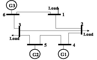
Figure 7. Test system
Method
Problem Formulation
The ORPD problem is to optimise the steady performance of a power system in terms of one or more objective functions while satisfying several equality and inequality constraints.
In this part, we suppose that the extremities FACTS devices are referred by bus i and j.
Objective functions
In this paper two objective functions are used:
Real power loss: This objective consists to minimise the real power loss PL in transmission lines that can be expressed as [1, 11]:
|
|
(14) |
|
|
(15) |

where: Nb : number of buses; Vk<αk and Vh<ah : respectively voltages at bus k and h; Ykh and qkh: respectively modulus and argument of the kh-th element of the nodal admittance matrix Y.
Voltage deviation: This objective is to minimize the deviation in voltage magnitude at load buses that can be expressed as:
|
|
(16) |
where: NL: number of load buses; ![]() : prespecified reference value of the
voltage magnitude at the i-th load bus;
: prespecified reference value of the
voltage magnitude at the i-th load bus; ![]() is
usually set to be 1.0 p.u.
is
usually set to be 1.0 p.u.
Problem Constraints
The problem constraints are divided to equality and inequality constraints.
Equality constraints
These represent typical load flow equations as follows:
|
|
(17) |
|
|
(18) |
where: PGi and QGi: generator real and reactive power at i-th bus, respectively; PDi and QGi: load real and reactive power at i-th bus, respectively; Gij and Bij: transfer conductance and susceptance between buses i and j, respectively.
Inequality constraints
These constraints can be summarized by:
Security constraints: These include the constraints of voltage at the i-th load buses VLi as follows:
|
|
(19) |
Parameters FACTS constraints:
|
rmin ≤ r ≤ rmax |
(20) |
|
γmin ≤ γ ≤ γmax |
(21) |
|
dmin ≤ d ≤ dmax |
(22) |
We should note that the vector of decision variables is U = [r, g, d].
Multi-Objective Optimization
In a MOP, there may not be one solution that is best with respect to all objectives. Usually, the aim is to determine the trade-off surface, which is a set of nondominated solution points, known as Pareto optimal solutions. Every individual in this set is an acceptable solution.
For any two X1 and X2, we can have one of two possibilities: one dominates the other or none dominates the other. In a minimization problem, we say that the solution X1 dominates X2, if the following two conditions are satisfied [13]:
|
|
(23) |
where Nobj: Number of objective functions and fi: i-th objective function.
The goal of a multi-objective optimization algorithm is not only to guide the search towards the Pareto optimal front, but, also to maintain population diversity in the set of the nondominated solutions.
In the rest of this section, we will present the elitist MOEA NSGAII. So, we must be start with a presentation of the NSGA approach.
NSGA approach: The basic idea behind NSGA is the ranking process executed before the selection operation. The ranking procedure consists to find the nondominated solutions in the current population P. These solutions represent the first front F1. Afterwards, this first front is eliminated from the population and the rest is processed in the same way to identify nondominated solutions for the second front F2. This process continues until the population is properly ranked. So, we can write [14]:
|
|
(24) |
where r is the number of fronts.
The same fitness value fk is assigned to all
of individuals of the same front Fk. This fitness value decreases
while passing from the front Fk to the Fk+1. To maintain
diversity in the population, a sharing method is used. Let consider dij
the variable distance (Euclidean norm) between two solutions ![]() and
and ![]() .
.
|
|
(25) |

where S is the number of variables in the MOP. The parameters ![]() and
and ![]() respectively
are the upper and lower bounds of variable Xk.
respectively
are the upper and lower bounds of variable Xk.
|
|
(26) |
The sharing procedure is as follows:
Step 1: Fix the niche radius sshare and a small positive number, e.
Step 2: Initiate fmin = Npop+e and the counter of front j =1.
Step 3: From the r nondominated fronts Fj which constitute P.
|
|
|
Step 4: For each individual ![]() :
:
§ associate the dummy fitness fj(q) = fmin - ε;
§ calculate the niche count ncq as given in [13];
§
calculate the shared fitness ![]()
 .
.
Step 5: ![]() and
j = j + 1.
and
j = j + 1.
Step 6: If j ≤ r, then, return to step 4. Else, the process is finished.
The MOEAs using nondominated sorting and sharing have been criticized mainly for their O(MN3) computational complexity (M is the number of objectives and N is the population size). Also, these algorithms are not elitist approaches and they need to specify the sharing parameter. To avoid these difficulties, we present in the following an elitist MOEA which is called Nondominated Sorting Genetic Algorithm II (NSGAII).
NSGAII approach: In this approach, the sharing function approach is replaced with a crowded comparison.
Initially, an offspring population Qt is created from the parent population Pt at the tth generation. After, a combined population Rt is formed [14].
![]()
Rt is sorted into different no domination levels Fj as shown in the NSGA approach. So, we can write:
![]()
where r is the number of fronts.
Finally, one iteration of the NSGAII procedure is as follows:
Step 1: Create the offspring population Qt from the current population Pt.
Step 2: Combine the two populations Qt and Pt to form Rt.
Step 3: Find the all nondominated fronts Fi and Rt.
Step 4: Initiate the new population Pt+1 = f and the counter of front for inclusion i = 1.
Step 5: While |Pt+1| + |Fi| ≤ Npop, do:
![]()
![]()
Step 6: Sort the last front Fi using the crowding distance in descending order and choose the first (Npop - |Pt+1|) elements of Fi.
Step 7: Use selection, crossover and mutation operators to create the new offspring population Qt+1 of size Nobj.
To estimate the density of solution surrounding a
particular solution ![]() in a nondominated
set F, we calculate the crowding distance as follows:
in a nondominated
set F, we calculate the crowding distance as follows:
Step 1: Let’s suppose q = |F|. For each
solution ![]() in F, set di = 0.
in F, set di = 0.
Initiate m = 1.
Step 2: Sort F in the descending order
according to the objective function of rank m. Let’s consider ![]() the vector of indices, i.e. Iim
is the index of the solution
the vector of indices, i.e. Iim
is the index of the solution ![]() in the
sorted list according to the objective function of rank m.
in the
sorted list according to the objective function of rank m.
Step 3: For each solution ![]() which verifies 2 ≤ Iim
≤ (q-1), update the value of di as follows:
which verifies 2 ≤ Iim
≤ (q-1), update the value of di as follows:
|
|
(27) |

Then, the boundary solutions in the sorted list (solutions with smallest and largest function) are assigned an infinite distance value, i.e. if, Iim = 1 or Imi = q, di = ∞.
Step 4: If m = M, the procedure is finished. Else, m = (m+1), and return to step 2.
Implementation of the NSGAII: The proposed NSGAII has been implemented using real-coded genetic
algorithm (RCGA) [14]. So, a chromosome X corresponding to a decision variable
is represented as a string of real values xi, i.e. X = x1x2…xlchrom.
lchrom is the chromosome size and xi is a real number within its
lower limit ai and upper limit bi. i.e. xi Î [ai,
bi]. Thus, for two individuals having as chromosomes respectively X
and Y and after generating a random number![]() ,
the crossover operator can provide two chromosomes X’ and Y’ with a probability
Pc as follows [14]:
,
the crossover operator can provide two chromosomes X’ and Y’ with a probability
Pc as follows [14]:
|
|
(28) |

In this study, the non-uniform mutation operator has
been employed. So, at the tth generation, a parameter xi
of the chromosome X will be transformed to other parameter ![]() with a probability Pm as follows:
with a probability Pm as follows:
|
|
(29) |
|
|
(30) |

where t is a random binary number, r is a random number ![]() and gmax is the maximum
number of generations. b is a positive constant chosen arbitrarily.
and gmax is the maximum
number of generations. b is a positive constant chosen arbitrarily.
Results and Discussion
The characteristics of lines and buses are marked in the Tables 1 and 2 respectively. These values are given in p.u. considering a base power of 100 MVA for the overall system and base voltages of 100 KV. The lower voltage magnitude limits at all buses are 0.9 p.u and the upper limits are 1.1 p.u. Three cases of power analysis are considered. Case 1 assumes the study without any compensation. Case 2 assumes an SSSC between two load buses. In case 3, an UPFC is assumed too between two load buses.
Table 1. Data lines
|
Line |
Impedance |
||
|
Bus i |
Bus j |
R |
X |
|
1 |
2 |
0.02 |
0.4 |
|
1 |
6 |
0.01 |
0.15 |
|
2 |
3 |
0.05 |
0.5 |
|
2 |
4 |
0.015 |
0.5 |
|
3 |
5 |
0.05 |
0.5 |
|
3 |
6 |
0.05 |
0.5 |
|
4 |
5 |
0.08 |
0.8 |
Table 2. Data buses
|
Bus |
V |
PG |
QG |
PD |
QD |
|
1 |
- |
0 |
0 |
0.840 |
0.500 |
|
2 |
- |
0 |
0 |
0.400 |
0.400 |
|
3 |
- |
0 |
0 |
0.96 |
0.300 |
|
4 |
1.025 |
0.200 |
- |
0.100 |
0.100 |
|
5 |
1.084 |
0.100 |
- |
0.100 |
0.100 |
|
6 |
1.000 |
- |
- |
0.100 |
0.100 |
Figure 8 shows the convergence characteristics of the load flow program after 6 iterations with a tolerance of 10-5.
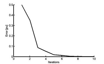
Figure 8. Convergence of the load flow
For the system without FACTS controllers, the voltage magnitude of load buses given by the load flow program, are not maintained within their permissible limits (Table 3). The corresponding values of voltage deviation and real power loss are respectively:
VD = 0.441 p.u. and PL = 0.133 p.u.
Table 3. Voltage magnitudes and phase angles for the system without FACTS controllers
|
Bus |
1 |
2 |
3 |
4 |
5 |
6 |
|
V |
0.828 |
0.868 |
0.947 |
1.025 |
1.084 |
1.00 |
|
α [rad] |
-0.299 |
-0.367 |
-0.195 |
-0.268 |
-0.141 |
0 |
Resolution of the ORPD
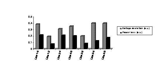
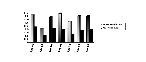
After execution of the optimization program, the values of the voltage deviation and the real power losses for the various positions of elements FACTS, are given in Figure 9.
(a) UPFC
(b) SSSC
Figure 9. The best position for system FACTS
Figure 9 shows that the best position of UPFC and SSSC for minimum voltage deviation and minimum real power loss, is in line 1-2. Therefore, we will give only the results corresponding to this optimal position.
Optimisation Mono-Objective
To get convergence of power loss and voltage deviation functions which are shown in Figures 10 and 11, these two objective functions are optimized individually.
Figure 10 shows the convergence of power losses function versus number of generations. From this Figure 10, we can see that a power losses corresponding to the two cases converge to 0.1322 p.u. and 0.1319 p.u., respectively, for the system with SSSC and with UPFC. And it shows that the UPFC corresponds to the best solution.
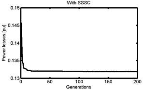
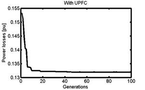
Figure 10. Convergence of power losses with generations
From Figure 11, we can see that voltage deviation corresponding to the two cases converges to 0.418 p.u. and 0.375 p.u., respectively, for the system with SSSC and with UPFC.
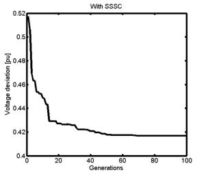
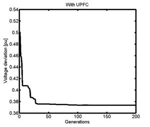
Figure 11. Convergence of voltage deviation with generations
Optimization Bi-Objective
In this section, the two objective functions are optimized simultaneously.
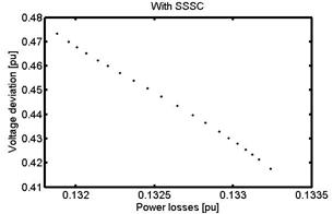
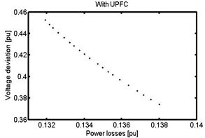
Figure 12. Pareto-optimal front of the proposed approach
Figure 12 gives the Pareto-optimal front corresponding to the two cases. And it shows that the UPFC corresponds to the best results.
Table 4. The best solution for voltage deviation
|
|
R |
g |
d |
VD |
Corresp. PL |
|
SSSC |
0.1525 |
1.253 |
0.442 |
0.418 |
0.133 |
|
UPFC |
0.1931 |
1.481 |
0.485 |
0.375 |
0.138 |
Table 5. The best solution for real power loss
|
|
R |
g |
d |
PL |
Corresp. VD |
|
SSSC |
0.1537 |
1.128 |
0.461 |
0.132 |
0.46 |
|
UPFC |
0.1952 |
1.369 |
0.527 |
0.132 |
0.45 |
After optimization by the NSGAII approach, we have obtained the Tables 4 and 5 giving the best solutions for minimum voltage deviation and minimum real power loss respectively.
The values of r, d, VD and PL are given in power units and g are in radians.
Table 6. For minimum voltage deviation
|
|
V1 [pu] |
V2 [pu] |
V3 [pu] |
|
SSSC |
0.9821 |
0.9274 |
0.9365 |
|
UPFC |
0.9915 |
0.9691 |
0.9467 |
Table 7. For minimum real power loss
|
|
V1 [pu] |
V1 [pu] |
V1 [pu] |
|
SSSC |
0.9778 |
0.9146 |
0.9217 |
|
UPFC |
0.9870 |
0.9541 |
0.9406 |
The profile voltage in load buses corresponding to the best solutions given in Tables 4 and 5 are shown respectively in Tables 6 and 7 and Vi is in power units. From tables 6 and 7, we can see that the voltage magnitude of load buses given witn FACTS are maintained within their permissible limits (0.9 pu<Vi<1.1 pu).
Conclusion
In this paper, a procedure based on MOEA to solve ORPD problem with FACTS was presented. This problem consists to minimize simultaneously real power loss in transmission lines and voltage deviation at load buses by using FACTS devices. The decision variables are parameters and location of FACTS devices.
The NSGAII approach is opted to solve this nonlinear MOP. UPFC and SSSC are used in this work. The resolution of the MOP shows that UPFC and SSSC have a positive effect on ORPD. Knowing that, UPFC gives the best results. The presented procedure was been tested on a 6-bus system.
References
4. Mishra S., Dash P.K., Hota P.K., Tripathy M., Genetically optimized neuro-fuzzy PFC for damping modal oscillations of power system, IEEE Transactions on Power Systems, 2002, 17(4), p. 1140-1147.
8. Zhang X.P., Advanced modelling of multicontrol functional static synchronous series compensator (SSSC) in Newton-Raphson power flow, IEEE Transactions on Power Systems, 2003, 18(4), p. 1410-1416.
11. Rubaai A., Villaseca F.E., Transient stability hierarchical control in multimachine power systems, IEEE Transactions on Power Systems, 1989, 4(4), p. 1438-1444.