Distributing Correlation Coefficients of Linear Structure-Activity/Property Models
Lorentz JÄNTSCHI 1, 2, and Sorana D. BOLBOACĂ 3, *
1 Technical University of
2
University of Agricultural Sciences and Veterinary Medicine
3 “Iuliu Haţieganu” University of Medicine
and Pharmacy
E-mail(s): lorentz.jantschi@gmail.com; sbolboaca@umfcluj.ro
* Corresponding author: Phone: +4-0264-431-697; Fax: +4-0264-593847
Abstract
Quantitative structure-activity/property relationships are mathematical relationships linking chemical structure and activity/property in a quantitative manner. These in silico approaches are frequently used to reduce animal testing and risk-assessment, as well as to increase time- and cost-effectiveness in characterization and identification of active compounds. The aim of our study was to investigate the pattern of correlation coefficients distribution associated to simple linear relationships linking the compounds structure with their activities. A set of the most common ordnance compounds found at naval facilities with a limited data set with a range of toxicities on aquatic ecosystem and a set of seven properties was studied. Statistically significant models were selected and investigated. The probability density function of the correlation coefficients was investigated using a series of possible continuous distribution laws. Almost 48% of the correlation coefficients proved fit Beta distribution, 40% fit Generalized Pareto distribution, and 12% fit Pert distribution.
Keywords
Probability density function; Determination coefficient; Quantitative Structure-Activity/Property Relationship (QSAR/QSPR); Molecular Descriptor Family on Vertices (MDFV).
Introduction
The probability density function of the correlation coefficient has previously been studied. Fisher studied the distribution law of correlation coefficient in samples drawn from large populations and obtained the exact sampling distribution of correlation coefficient [1]. Furthermore, Fisher proved that the correlation coefficient in the sample (abbreviated as 'r') is greater than the correlation coefficient in the population (abbreviated as 'ρ') [1]. Therefore, it is consider that the sample correlation coefficient is a biased estimator of the population correlation coefficient; the bias decreases as sample size increases and becomes 0 when the population correlation coefficient is 0 [2]. The use of unbiased estimators for population correlation coefficient is recommended in the specialty literature (for example the Fisher's formula: ρEst = r/[1+(1-r2)/2] [1] – where r2 is determination coefficient – or Olkin and Pratt formula ρEst = r/{1+(1-r2)/[2•(n-3)]} [3] – where n is the sample size. Pearson investigated the distribution frequency of correlation coefficients in sample sizes of 20 and 30 measurements [4]. Similar research studies were conducted on small sample sizes (< 20 observations) extracted from normal or non-normal populations and either good or bad agreement with theoretical distribution was identified or not [5-7].
Structure activity/property relationship approaches (statistical models able to link the compound structure with their activity/property) have been introduced as competent modeling methods able to reduce animal testing and risk-assessment, as well as to increase time- and cost-effectiveness by guiding the selection for compounds for in vivo testing [8]. Various approaches are available for identifying descriptors based on the structure of compounds, such as comparative molecular field analysis [9], Hansch analysis [10], quantitative neighborhoods of atoms [11], minimum topological difference [12], comparative molecular field analysis and comparative molecular similarity index analysis [13], bond-level molecular descriptors [14], conformational sample pharmacophore [15], linear expression by representative energy terms [16], Molecular Descriptors Family [17, 18] Molecular Descriptors Family on Vertices [19,20], characteristic and/or counting polynomials [21], etc. The most frequently used statistical approaches used to identify the link between the structure of compounds and their activity/property include linear regression as complete search [22-24] or heuristic search [25-28], self-consistent regression [29], logistic regression [30,31], partial least squares [32,33], principal component analysis [33,34], cluster analysis [30,35], discriminant analysis [30,36].
Correlation coefficient and leave-one-out correlation coefficient are the most frequently empirical measures of the goodness-of-fit of any QSAR (quantitative structure-activity relationship) or QSPR (quantitative structure-property relationship) model. The threshold value for correlation coefficient is 0.6 while the threshold value for leave-one-out correlation coefficient is 0.5 [37]. Any model with both correlation coefficient and leave-one-out correlation coefficient that exceed these thresholds are considered good models. To date, we have found no studies that assess the probability density function of correlation coefficients. In consequence, we decide to look closer on this problem.
The aim of our study was to investigate the pattern of the distribution law for correlation coefficient in simple linear regressions that was applied to the structure-activity/property relationships for thirty-one activities/properties of a small sample data set of ordnance compounds.
Material and Method
Compounds and Toxicities
A sample of eight ordnance compounds with a range of toxicities on Arbacia punctulata (sea urchin), Dinophilus gyrociliatus (polychaete), Sciaenops ocellatus (redfish), Opossum shrimp (mysid), and Ulva fasciata (macro-alga) species was included in the study. The measurements were taken from literature [38]. Nine half maximal effective concentrations (EC50), eight lowest observed effect concentrations (LOEC), seven no observed effect concentrations (NOEC), six energies, and dipole moment (computed with HyperChem - v. 8, Hypercube Inc., USA) were investigated (Table 1).
The PubChem database was used to download the structure as structure data format file (*.sdf). A program made by authors was used to convert the *.sdf files into HyperChem file (*.hin) to prepare the molecules for modeling. A logarithmic transformation was applied on observed/measured toxicities and calculated properties to assure the normality of data, criterion needed to conduct the linear regression analysis [39,40].
Table 1. Ordnance compounds and associated toxicities / properties.
|
CID Act/Prop |
8461a |
11813b |
8376c |
7452d |
7434e |
8490f |
10178g |
6954h |
|
EC50SF |
68.00 |
n.a. |
258.00 |
84.00 |
n.a. |
n.a. |
3.00 |
349.00 |
|
EC50SED |
51.40 |
6.70 |
12.00 |
92.00 |
1.30 |
n.a. |
0.08 |
281.00 |
|
EC50AS |
2.50 |
6.70 |
2.50 |
0.85 |
0.08 |
12.00 |
0.67 |
415.00 |
|
EC50AGL |
1.70 |
2.90 |
0.76 |
0.41 |
0.05 |
8.10 |
0.34 |
94.00 |
|
EC50AGCN |
2.10 |
4.20 |
1.40 |
0.45 |
0.06 |
9.80 |
0.40 |
118.00 |
|
EC50LS |
21.00 |
13.00 |
7.70 |
15.00 |
2.10 |
n.a. |
0.06 |
265.00 |
|
EC50PL |
5.70 |
2.10 |
1.80 |
3.70 |
0.60 |
26.00 |
0.02 |
155.00 |
|
EC50RLs |
48.00 |
34.00 |
8.20 |
46.00 |
1.40 |
n.a. |
1.80 |
127.00 |
|
EC50MS |
5.40 |
5.60 |
0.98 |
7.10 |
1.30 |
n.a. |
1.30 |
13.00 |
|
NOECSF |
39.00 |
23.00 |
103.00 |
84.00 |
35.00 |
n.a. |
75.00 |
178.00 |
|
NOECSED |
18.00 |
n.a. |
2.10 |
n.a. |
0.24 |
75.00 |
0.04 |
178.00 |
|
NOECSG |
0.94 |
2.20 |
1.70 |
0.30 |
0.05 |
9.20 |
0.50 |
169.00 |
|
NOECAS |
9.50 |
14.60 |
6.10 |
9.70 |
1.20 |
49.00 |
0.03 |
199.00 |
|
NOECAGL |
n.a. |
n.a. |
1.40 |
2.40 |
0.35 |
11.90 |
0.02 |
108.00 |
|
NOECRLs |
34.60 |
13.70 |
6.30 |
25.20 |
0.99 |
68.00 |
1.20 |
97.00 |
|
NOECMS |
3.60 |
5.00 |
0.65 |
5.20 |
0.96 |
47.00 |
1.10 |
9.20 |
|
LOECSF |
75.00 |
45.00 |
n.a. |
110.00 |
48.00 |
n.a. |
0.60 |
352.00 |
|
LOECSED |
39.00 |
5.00 |
9.10 |
84.00 |
0.48 |
n.a. |
0.08 |
352.00 |
|
LOECSG |
1.80 |
4.70 |
3.40 |
0.65 |
0.09 |
15.70 |
1.00 |
336.00 |
|
LOECAGL |
0.48 |
1.20 |
0.21 |
0.21 |
0.05 |
5.00 |
0.25 |
92.00 |
|
LOECAS |
19.00 |
29.60 |
11.60 |
19.60 |
2.40 |
n.a. |
0.06 |
379.00 |
|
LOECPL |
2.40 |
1.80 |
2.80 |
4.40 |
0.61 |
23.70 |
0.03 |
198.00 |
|
LOECRLs |
66.80 |
32.00 |
10.80 |
49.60 |
2.00 |
n.a. |
2.60 |
187.00 |
|
LOECMS |
6.80 |
9.80 |
1.34 |
9.70 |
1.88 |
n.a. |
2.00 |
20.60 |
|
OPLSSAE |
-59574 |
-59574 |
-78558 |
-56262 |
-75246 |
-81679 |
-102472 |
-82536 |
|
OPLSSBE |
-1947 |
-1942 |
-2111 |
-1665 |
-1833 |
-1756 |
-2474 |
-1937 |
|
OPLSSCE |
226212 |
229560 |
324933 |
192456 |
282678 |
356017 |
465605 |
327194 |
|
OPLSSEE |
-287733 |
-291075 |
-405601 |
-250382 |
-359757 |
-439452 |
-570551 |
-411667 |
|
OPLS_DM |
5.43 |
3.51 |
1.52 |
4.84 |
0.00 |
6.97 |
2.85 |
1.53 |
|
OPLS_HF |
25.97 |
31.15 |
42.38 |
32.95 |
44.67 |
104.87 |
23.79 |
0.96 |
|
OPLS_TE |
-61521 |
-61516 |
-80668 |
-57927 |
-77079 |
-83435 |
-104947 |
-84472 |
|
CID = Chemical IDentifier (PubChem, http://pubchem.ncbi.nlm.nih.gov/); Prop = property; IUPACs: a = 1-methyl-2,4-dinitrobenzene; b = 2-methyl-1,3-dinitrobenzene; c = 2-methyl-1,3,5-trinitrobenzene; d = 1,3-dinitrobenzene; e = 1,3,5-trinitrobenzene; f = 1,3,5-trinitro-1,3,5-triazinane; g = N-methyl-N-(2,4,6-trinitrophenyl)nitramide; h = 2,4,6-trinitrophenol; EC50 (half maximal effective concentration) = the effective concentration of toxin in aqueous solution that produces a specific measurable effect in 50% of the test organisms within the stated study time; SF = Arbacia punctulata fertilization; SED = Arbacia punctulata embryological development; AS = Ulva fasciata survival; AGL = Ulva fasciata germling length; AGCN = Ulva fasciata germling cell number; LS = Sciaenops ocellatus larvae survival; PL = Dinophilus gyrociliatus laid eggs/female; RLs = Sciaenops ocellatus larvae survival; MS = Opossum shrimp juveniles survival; SG = Arbacia punctulata germination; NOEC (No Observed Effect Concentration) = highest concentration of toxicant to which organisms are exposed in a full or partial life-cycle test, that determine no observable adverse effects on the test organisms; LOEC (Lowest Observed Effect Concentration) = lowest concentration of toxicant to which organisms are exposed in a full or partial life-cycle test, which causes adverse effects on the test organisms; OPLSSAE = isolated atom energy from semi-empirical method; OPLSSBE = energy relative to isolated atoms; OPLSSCE = core-core interaction energy; OPLSSEE = electronic energy for a semi-empirical calculation; OPLS_DM = dipole-moment; OPLS_HF = heat-of-formation; OPLS_TE = total-energy; n.a. = not available. |
||||||||
Descriptor Calculations and Models Identification
The workflow applied for compounds modeling and probability density function analysis is briefly presented in Figure 1.
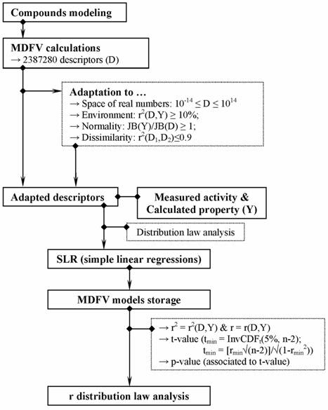
Figure 1. Workflow of analysis of probability density function of correlation coefficients (where InvCDF = inverse cumulative distribution function; D = descriptor; Y = observed activity / calculated property; JB = Jarque Berra statistic (Jarque and Bera, 1981); n = sample size; CV = coefficient of variation; r2 = determination coefficient; r = correlation coefficient; min = minimum value).
Ordnance compounds modeling represented first step in our analysis. The 3D structure of the molecules was created and geometrically optimized using HyperChem. The geometry of compounds was optimized by applying the Austin method [41], Polak-Ribiere algorithm using a program made by one of the authors [42].
Calculation of MDFV descriptors represented the second step conducted in our analysis. The structural information of investigated ordnance compounds was translated into molecular descriptors using the MDFV approach (Molecular Descriptors Family on Vertices cut, first reported in [19]). MDFV is a method based on vertices that implement 8 features as detailed in Table 2.
Table 2. Feature of the MDFV descriptors.
|
Feature |
No. |
Space |
Remarks / Values |
|
Distance metric |
2 |
{T, G} |
Values: T (topological distance), G (geometric distance) |
|
Atomic property |
7 |
{C, H, M, E, Q, L, A} |
Values: C (cardinality), H (number of hydrogen atoms adjacent to the investigated atom), M (relative atomic mass), E (electronegativity), Q (atomic partial charge, Extended Hückel energy [20]), L (melting point under normal temperature and pressure conditions), A (electronic affinity) |
|
Interaction operator |
58 |
{J, j, O, o, P, p, Q, q, R, r, K, k, L, l, M, m, N, n, W, w, X, x, Y, y, Z, z, S, s, T, t, U, u, V, v, F, f, G, g, H, h, I, i, A, a, B, b, C, c, D, d, 0, 1, 2, 3, 4, 5, 6, 7} |
Values: J=D, j=1/D, O=P1, o=1/P1, P=P2, p=1/P2, Q=P1P2, q=1/P1P2, R=√(P1P2), r=1/√(P1P2), K=P1D, k=(1/P1)D, L=P2D, l=(1/P2)D, M=P1P2D, m=(1/P1P2)D, N=√(P1P2)D, n=(1/√(P1P2))D, W=P1D2, w=(1/P1)D2, X=P2D2, x=(1/P2)D2, Y=P1P2D2, y=(1/P1P2)D2, Z=√(P1P2)D2, z=(1/√(P1P2))D2, S=P1/D, s=(1/P1)/D, T=P2/D, t=(1/P2)/D, U=P1P2/D, u=(1/P1P2)/D, V=√(P1P2)/D, v=(1/√(P1P2))/D, F=P1/D2, f=(1/P1)/D2, G=P2/D2, g=(1/P2)/D2, H=P1P2/D2, h=(1/P1P2)/D2, I=√(P1P2)/D2, i=(1/√(P1P2))/D2, A=P1/D3, a=(1/P1)/D3, B=P2/D3, b=(1/P2)/D3, C=P1P2/D3, c=(1/P1P2)/D3, D=√(P1P2)/D3, d=(1/√(P1P2))/D3, 0=P1/D4, 1=(1/P1)/D4, 2=P2/D4, 3=(1/P2)/D4, 4=P1P2/D4, 5=(1/P1P2)/D4, 6=√(P1P2)/D4, 7=(1/√(P1P2))/D4, where D = distance operator and P = atomic property |
|
Overlapping interaction at fragment/vertices level |
7 |
{A, a, I, i, F, P, C } |
Values: A (maximum value), a (maximum value of the sum of squares on the X, Z, and Y projections), I (minimum value), i (minimum value of the sum of squares on the X, Z, and Y projections), F (projection overlaps on axes), P (mediate the unity value of the descriptor on the X, Z, or Y projections and overlap the descriptors values), C (aggregate value in the center of descriptor) |
|
Overlapping interaction at molecule level |
7 |
{A, a, I, i, F, P, C } |
|
|
Interaction for each overlap and per atom/fragment |
10 |
{f, F, c, C, p, P, a, A, i, I} |
Values: f (vectorial overlap of descriptors per fragment), F (vectorial overlap of descriptor per atom), c (aggregate in the center of descriptor per fragment), C (aggregate in the center of descriptor per atom), p (mediates the unity value of the descriptor on the X, Z, or Y projections and overlaps the descriptors values per fragments), P (mediates the unity value of the descriptor on the X, Z, or Y projections and overlaps the descriptors values per atom), a (absolute maximum value of descriptors - interactions in the fragment), A (absolute maximum value of descriptors - interaction of the fragment with the atom), i (absolute minimum value of descriptors - interactions in the fragment), I (absolute minimum value of descriptors - interaction of the fragment with the atom) |
|
Expression unit |
2 |
{D, d} |
Values: D (value of molecular descriptor), d (value of the descriptor projection on the X, Z, and Y axes) |
|
Linearization operator |
3 |
{I, R, L} |
Values: I (identity), R (reciprocal), L (logarithm) |
The MDFV family comprises 2387280 descriptors (2×7×58×7×7×10×2×3) for any sample of compounds [19,20]. Filtration of the MDFV descriptors in order to obtain the pool of adapted descriptors represented the third step in our analysis. The following properties defined an adapted descriptor:
§ (be "alive"): Real descriptor values for all compounds in the data set (the imposed range was from 10-14 to 1014).
§ (be "useful"): Variability-Determination-Normality. The variability was defined as CV(D) ≥ 10%·CV(Y), where CV = coefficient of variation, D = value of descriptor, Y = value of observed/measured/calculated activity/property. Determination was defined as r2(D,Y) ≥ 0.10, where r2 = determination coefficient, while normality was defined using the criterion - JB(D) ≥ JB(Y), where JB = Jarque Berra statistic.
§ (be "unique"): Distinct τc(D,Y) or r2(D1,D2) ≤ 0.9, where τc = Kendall tau c correlation coefficient [44].
All descriptors that accomplished simultaneously the above-presented criteria and had a high determination coefficient calculated between value of descriptor and activity/property were included in the pool of adapted descriptors. The search space was furthermore limited from adapted descriptors to probable descriptors. A probable descriptor was defined as that descriptor able to correlate enough with activity/property under the assumption of simple linear association hypothesis (non-zero correlation coefficient) at a significance level of 5%. Probable descriptors were obtained in the fourth step of our analysis.
The obtained QSAR/QSPR linear models were stored in a database and were classified according to the value of correlation coefficient r(Y,Ŷ) (where , r=r(Y,Ŷ)=|r(Y,D)|, Y = measured activity / calculated property, Ŷ = estimated activity/property, Ŷ=a·D+b - D = value of MDFV descriptor, a and b = coefficient of the simple linear regression). The following data were stored for each model: value of correlation (r(Y,Ŷ)) and determination coefficient (r2(Y,Ŷ)), t-value associated to significance of regression coefficients (tmin = InvCDFStudent_t(5%, n-2), where InvCDF = inverse of cumulative distribution function; n = sample size), and the probability associated to t-value (p-value).
Investigation of the Distribution Law
Distribution function of the obtained correlation coefficients was conducted at a significance level of 1% in the fifth step of our analysis. A search for continuous distribution functions was conducted on correlation coefficients (EasyFit Professional, version 5.1, MathWave Technologies). Kolmogorov-Smirnov [45] (abbreviated as K-S), Anderson-Darling [46] (abbreviated as A-D) and/or Chi-Squared [47] (abbreviated C-S) statistics were used to measure the departure between observation and a theoretical probability density function (PDF). Fisher method (Fisher's Chi-Squared, abbreviated as F-C-S) was used to identify the most suitable distribution law [48].
Results and Discussion
The population of adapted descriptors was obtained for the investigated ordnance compounds starting from the pool of the 2387280 MDFV descriptors. The number of adapted descriptors varied from 0.01% (for LOEC(PL) - lowest observed effect concentration of polychaete laid eggs/female) to 0.55% (for OPLSSBE - energy relative to isolated atoms) (see Table 3).
Table 3. MDFV descriptors: from adapted descriptors to probable descriptors.
|
Act/Prop |
No of adapted descriptors |
No of probable descriptors |
n |
|
Act/Prop |
No of adapted descriptors |
No of probable descriptors |
n |
|
EC50AS |
1778 |
218 |
8 |
|
LOECSG |
1902 |
183 |
8 |
|
EC50AGCN |
579 |
71 |
8 |
|
NOECAGL |
1796 |
171 |
8 |
|
EC50AGL |
824 |
102 |
8 |
|
NOECMS |
2403 |
515 |
8 |
|
EC50LS |
3754 |
546 |
7 |
|
NOECPL |
382 |
43 |
6 |
|
EC50MS |
5329 |
818 |
7 |
|
NOECAS |
9417 |
1154 |
8 |
|
EC50PL |
944 |
208 |
8 |
|
NOECRLs |
4167 |
559 |
8 |
|
EC50RLs |
4908 |
702 |
7 |
|
NOECSED |
2550 |
275 |
6 |
|
EC50SED |
3588 |
478 |
7 |
|
NOECSF |
1255 |
37 |
7 |
|
EC50SF |
2262 |
179 |
5 |
|
OPLSSAE |
2466 |
800 |
8 |
|
LOECAGL |
6447 |
647 |
8 |
|
OPLSSBE |
13060 |
2801 |
8 |
|
LOECAS |
5270 |
764 |
7 |
|
OPLSSCE |
4847 |
1543 |
8 |
|
LOECMS |
4444 |
637 |
7 |
|
OPLSSEE |
4309 |
1403 |
8 |
|
LOECPL |
165 |
38 |
8 |
|
OPLS_HF |
1485 |
308 |
8 |
|
LOECRLs |
3285 |
431 |
7 |
|
OPLS_TE |
2484 |
781 |
8 |
|
LOECSED |
2484 |
294 |
7 |
|
OPLS_DM |
3917 |
722 |
8 |
|
LOECSF |
7169 |
946 |
6 |
|
|
|
|
|
|
EC50 (half maximal effective concentration) = the effective concentration of toxin in aqueous solution that produces a specific measurable effect in 50% of the test organisms within the stated study time; NOEC (No Observed Effect Concentration) = highest concentration of toxicant to which organisms are exposed in a full or partial life-cycle test, that determine no observable adverse effects on the test organisms; LOEC (Lowest Observed Effect Concentration) = lowest concentration of toxicant to which organisms are exposed in a full or partial life-cycle test, which causes adverse effects on the test organisms; n = sample size; AS = Ulva fasciata survival; AGCN = Ulva fasciata germling cell number; AGL = Ulva fasciata germling length; LS = Sciaenops ocellatus larvae survival; MS = Opossum shrimp juveniles survival; PL = Dinophilus gyrociliatus laid eggs/female; RLs = Sciaenops ocellatus larvae survival; SED = Arbacia punctulata embryological development; SF = Arbacia punctulata fertilization; SG = Arbacia punctulata germination; OPLSSAE = isolated atom energy from semi-empirical method; OPLSSBE = energy relative to isolated atoms; OPLSSCE = core-core interaction energy; OPLSSEE = electronic energy for a semi-empirical calculation; OPLS_DM = dipole-moment; OPLS_HF = heat-of-formation; OPLS_TE = total-energy |
||||||||
The adapted descriptors (the sample containing all thirty-one investigated activities and properties) proved fit Fisher-Tippett (Figure 2), as this distribution law was neither rejected by any of the three used statistics nor by the overall statistic (Fisher's Chi-Squared statistic, Table 4). Fisher-Tippett distribution [49] is an extreme value distribution on independent and identically distributed random variables on large sample sizes (e.g. thousands observations).
Table 4. Fisher-Tippett distribution fit the number of adapted descriptors?
|
Statistic |
Statistic-value |
p-value |
|
0.0804 |
0.9786 |
|
|
Anderson-Darling |
0.1545 |
0.8750 |
|
Chi-Squared |
1.0324 |
0.9049 |
|
0.2551 |
0.9682 |
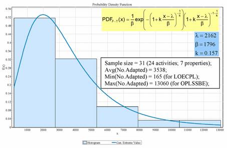
Figure 2. Fisher-Tippett distribution for number of adapted descriptors (x = number of adapted descriptors; f(x) = probability density function; Avg = arithmetic mean; Min= minimum; Max = maximum; λ, β, and k = parameters of Fisher-Tippett distribution; LOECPL = Lowest Observed Effect Concentration - Dinophilus gyrociliatus laid eggs/female; OPLSSBE = energy relative to isolated atoms).
The number of probable descriptors varied from 2.95% (for NOEC(SF) - no observed effect concentration of sea urcin fertilization) to 32.56% (for OPLSSEE - electronic energy for a semi-empirical calculation) relative to the number of adapted descriptors. Fisher-Tippet distribution law was identified the most suitable also for probable descriptors (Figure 3). The Fisher-Tippet distribution of probable descriptors was neither rejected by any of the three used statistics nor by the Fisher's Chi-Squared statistic (Table 5).
Table 5. Fisher-Tippett distribution fit the number of probable descriptors?
|
Statistic |
Statistic-value |
p-value |
|
Kolmogorov-Smirnov |
0.0831 |
0.9708 |
|
Anderson-Darling |
0.3105 |
0.7410 |
|
Chi-Squared |
2.7506 |
0.4317 |
|
Fisher's Chi-Squared |
1.1694 |
0.7604 |
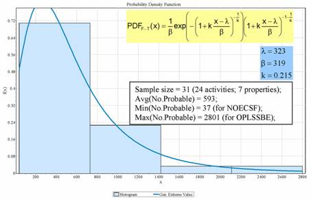
Figure 3. Fisher-Tippett distribution law for number of probable descriptors (x = number of probable descriptors; f(x) = probability density function; Avg = arithmetic mean, Min= minimum; Max = maximum; λ, β, and k = parameters of Fisher-Tippett distribution; NOECSF = No Observed Effect Concentration of Arbacia punctulata fertilization; OPLSSBE = energy relative to isolated atoms).
The probability sub-space of probable descriptors was obtained from the probability distribution laws of both adapted and probable descriptors (coordinates: probability vs. number of descriptors, Figure 4). The probability sub-space of probable descriptors must be located under one of the Probable(x)/q curves (where q = a quantity that must be estimated) which is located under the probability curve of the adapted descriptors (Adapted(x)) (Figure 4). Probable(x)/6, Probable(x)/9 and Probable(x)/12 curves were obtained taking into consideration that probable descriptors are a subset of adapted descriptors, which is also reflected in the probability space (Adapted(x)=CDFF-T(x) for PDFF-T(x) in Figure 2, and Adapted(x)=CDFF-T(x) for PDFF-T(x) in Figure 3).
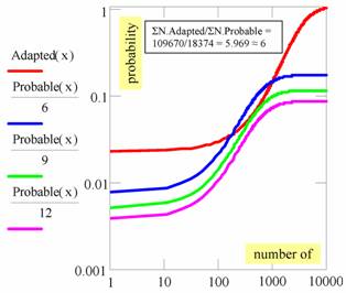
Figure 4. Probability space of adapted and probable descriptors.
The first probability density function lower than the probability density function of adapted descriptors is Probable(x)/9 as seen in Figure 4. The probability density function of Probable(x)/6 is over the probability density function of Adapted(x), which could be explained by Fisher’s rule regarding the correlation coefficient "r generally greater than ρ" [1]. Thus, almost 33% of correlation coefficients from "probable" descriptors had greater values than the threshold value while the ρ values (true correlation values in the population) were smaller than the threshold value (critical 0.05% value - Student t distribution). Therefore, almost 33% of regressions/correlations passed the Student t-test (statistically significant correlation coefficients). However, this does not mean that they are real models of associations (not statistically significant ρ values).
Several distribution laws were identified as being most suitable for the correlation coefficients: Beta, Fisher-Tippett, Generalized Logistic, Generalized Pareto, Johnson SB, Kumaraswamy, Log-Pearson 3, Pert, Power Function, Reciprocal, Triangular, Uniform, and Wakeby. The analysis of suitability of above-presented distribution laws at a significance level of 0.1% are presented in Table 6 for investigated properties and in Table 7 for investigated activities. The properties were not further investigated with regard to the distribution of the correlation coefficients since no agreement was identified when distribution laws of correlation coefficient in structure-property models were analyzed (see Table 6). This was the reason why the properties were no further investigated.
Table 6. Distribution laws of correlation coefficient (α = 0.1%): properties of ordnance compounds.
|
Prop |
OPLSSAE |
OPLSSBE |
OPLSSCE |
OPLSSEE |
OPLS_DM |
OPLS_HF |
OPLS_TE |
|
Beta |
1 |
0 |
0 |
1 |
0 |
0 |
1 |
|
Fisher-Tippett |
0 |
0 |
0 |
0 |
0 |
0 |
0 |
|
Gen. Logistic |
0 |
0 |
0 |
0 |
0 |
0 |
0 |
|
Gen. Pareto |
0 |
0 |
0 |
0 |
0 |
0 |
0 |
|
Johnson SB |
0 |
1 |
0 |
0 |
0 |
0 |
0 |
|
Kumaraswamy |
0 |
0 |
1 |
1 |
1 |
0 |
1 |
|
Log-Pearson 3 |
0 |
0 |
0 |
0 |
0 |
0 |
0 |
|
Pert |
0 |
0 |
0 |
0 |
0 |
0 |
0 |
|
Power Function |
0 |
0 |
0 |
0 |
0 |
0 |
0 |
|
Reciprocal |
0 |
0 |
0 |
0 |
0 |
0 |
0 |
|
Triangular |
0 |
1 |
0 |
0 |
0 |
0 |
0 |
|
Uniform |
0 |
0 |
0 |
0 |
0 |
0 |
0 |
|
Wakeby |
0 |
0 |
0 |
0 |
1 |
0 |
0 |
|
1 = fit; 0 = not fit; PDF = probability density function; Gen. Logistic = Generalized Logistic; Gen. Pareto = Generalized Pareto; OPLSSAE = isolated atom energy from semi-empirical method; OPLSSBE = energy relative to isolated atoms; OPLSSCE = core-core interaction energy; OPLSSEE = electronic energy for a semi-empirical calculation; OPLS_DM = dipole-moment; OPLS_HF = heat-of-formation; OPLS_TE = total-energy; n.a. = not available |
|||||||
Table 7. Distribution law of correlation coefficients: activities of ordnance compounds.
|
|
EC50SF |
EC50SED |
EC50AS |
EC50AGL |
EC50AGCN |
EC50LS |
EC50PL |
EC50RLs |
EC50MS |
NOECSF |
NOECSED |
NOECSG |
NOECAS |
NOECPL |
NOECRLs |
NOECMS |
LOECSF |
LOECSED |
LOECSG |
LOECAGL |
LOECAS |
LOECPL |
LOECRLs |
LOECMS |
∑ |
|
Beta |
1 |
0 |
1 |
1 |
1 |
0 |
1 |
1 |
0 |
1 |
1 |
0 |
1 |
1 |
1 |
1 |
0 |
0 |
1 |
1 |
0 |
1 |
1 |
0 |
16 |
|
Fisher-Tippett |
1 |
1 |
1 |
0 |
0 |
0 |
0 |
0 |
1 |
0 |
0 |
0 |
1 |
0 |
0 |
0 |
1 |
1 |
1 |
1 |
0 |
1 |
1 |
1 |
12 |
|
Gen. Logistic |
1 |
1 |
1 |
0 |
0 |
0 |
0 |
0 |
1 |
0 |
0 |
0 |
1 |
0 |
0 |
0 |
1 |
1 |
0 |
1 |
0 |
0 |
0 |
0 |
8 |
|
Gen. Pareto |
0 |
1 |
1 |
0 |
1 |
1 |
0 |
0 |
1 |
0 |
1 |
1 |
1 |
1 |
1 |
0 |
0 |
0 |
0 |
1 |
1 |
0 |
1 |
1 |
14 |
|
Johnson SB |
1 |
1 |
1 |
0 |
1 |
1 |
1 |
1 |
1 |
1 |
0 |
1 |
0 |
1 |
0 |
1 |
0 |
1 |
1 |
1 |
1 |
1 |
1 |
0 |
18 |
|
Kumaraswamy |
1 |
0 |
1 |
0 |
0 |
0 |
1 |
0 |
0 |
1 |
1 |
0 |
1 |
1 |
0 |
0 |
1 |
1 |
0 |
0 |
0 |
1 |
0 |
0 |
10 |
|
Log-Pearson 3 |
1 |
1 |
1 |
0 |
0 |
0 |
0 |
0 |
1 |
0 |
0 |
0 |
1 |
0 |
0 |
0 |
1 |
1 |
1 |
1 |
0 |
1 |
1 |
0 |
11 |
|
Pert |
1 |
1 |
0 |
0 |
0 |
0 |
1 |
1 |
1 |
1 |
0 |
0 |
1 |
1 |
1 |
0 |
1 |
1 |
1 |
1 |
0 |
1 |
1 |
0 |
15 |
|
Power Function |
0 |
1 |
0 |
0 |
0 |
0 |
0 |
0 |
0 |
0 |
0 |
0 |
1 |
0 |
0 |
0 |
0 |
0 |
0 |
1 |
0 |
0 |
0 |
1 |
4 |
|
Reciprocal |
0 |
0 |
0 |
0 |
0 |
0 |
0 |
0 |
0 |
0 |
0 |
0 |
1 |
0 |
0 |
0 |
0 |
0 |
0 |
1 |
0 |
0 |
0 |
0 |
2 |
|
Triangular |
1 |
1 |
1 |
0 |
0 |
1 |
0 |
1 |
1 |
0 |
1 |
1 |
1 |
1 |
1 |
1 |
0 |
0 |
0 |
1 |
0 |
1 |
1 |
0 |
15 |
|
Uniform |
0 |
0 |
0 |
0 |
0 |
0 |
0 |
0 |
0 |
0 |
0 |
0 |
0 |
0 |
0 |
0 |
0 |
0 |
0 |
1 |
0 |
0 |
0 |
0 |
1 |
|
Wakeby |
1 |
1 |
1 |
0 |
1 |
0 |
0 |
0 |
0 |
0 |
0 |
0 |
1 |
1 |
1 |
1 |
0 |
0 |
1 |
1 |
0 |
0 |
0 |
1 |
11 |
|
1 = fit; 0 = not fit; EC50 (half maximal effective concentration) = the effective concentration of toxin in aqueous solution that produces a specific measurable effect in 50% of the test organisms within the stated study time; SF = Arbacia punctulata fertilization; SED = Arbacia punctulata embryological development; AS = Ulva fasciata survival; AGL = Ulva fasciata germling length; AGCN = Ulva fasciata germling cell number; LS = Sciaenops ocellatus larvae survival; PL = Dinophilus gyrociliatus laid eggs/female; RLs = Sciaenops ocellatus larvae survival; MS = Opossum shrimp juveniles survival; SG = Arbacia punctulata germination; NOEC (No Observed Effect Concentration) = highest concentration of toxicant to which organisms are exposed in a full or partial life-cycle test, that determine no observable adverse effects on the test organisms; LOEC (Lowest Observed Effect Concentration) = lowest concentration of toxicant to which organisms are exposed in a full or partial life-cycle test, which causes adverse effects on the test organisms; |
|||||||||||||||||||||||||
Nine distribution laws out of 13 proved to be suitable for defining the correlation coefficients for quantitative structure-activity models (Table 7). The following distribution laws were withdrawn from the analysis since their results in terms of fit were covered by other distribution laws: Uniform (Uniform Í Triangular), Generalized logistic (Generalized Logistic Í Fisher-Tippett), and Reciprocal and Power probability density functions (Reciprocal Í Power Function Í Generalized Pareto).
The smallest set of distribution laws able to cover (maximum in convergence) the investigated activities of ordnance compounds was searched. No pairs of PDFs able to cover the distribution laws of correlation coefficients for QSARs models were identified. The largest coverage was provided by Generalized Pareto & Johnson SB; Generalized Pareto & Pert; Generalized Pareto & Beta; and Beta & Johnson SB, but in all cases at least two no fit were presented (Table 7). The following sets of three distribution laws could be suitable alternatives since they are able to cover the space of the investigated toxicities of ordnance compounds (Table 8): Beta & Fisher-Tippett & Generalized Pareto, Beta & Fisher-Tippett & Johnson SB, Beta & Generalized Pareto & Kumaraswamy, Beta & Generalized Pareto & Log-Pearson 3; and Beta & Generalized Pareto & Pert. A detailed analysis could be found in Supplementary Material.
Table 8. Joined probability density functions (PDFs): summary statistic and overall probability.
|
PDFs association |
Parameters (Param) |
∑ |
Agreements (Agr) |
∑ |
Agr/Param |
Joined F-C-S value (df=24)/p |
||||
|
Beta & Fisher-Tippett & Generalized Pareto |
4 |
3 |
3 |
10 |
16 |
12 |
14 |
42 |
4.20 |
5.486/0.999969 |
|
Beta & Fisher-Tippett & Johnson SB |
4 |
3 |
4 |
11 |
16 |
12 |
18 |
46 |
4.18 |
4.677/0.999993 |
|
Beta & Generalized Pareto & Kumaraswamy |
4 |
3 |
4 |
11 |
16 |
14 |
10 |
40 |
3.64 |
8.092/0.998993 |
|
Beta & Generalized Pareto & Log-Pearson 3 |
4 |
3 |
3 |
10 |
16 |
14 |
11 |
41 |
4.10 |
5.933/0.999936 |
|
Beta & Generalized Pareto & Pert |
4 |
3 |
3 |
10 |
16 |
14 |
15 |
45 |
4.50 |
6.854/0.999760 |
|
F-C-S = Fisher’s Chi-Squared; df = degrees of freedom; p = probability |
||||||||||
The analysis of the results presented in Table 8 reveals the following:
§ Beta & Generalized Pareto & Pert is the most suitable for correlation coefficients of QSAR models both in terms of agreements and parameters ratio (the ratio had the highest value). Therefore, the results presented in Table 8 reveal that Beta & Generalized Pareto & Pert association could comprise the distribution laws for the correlation coefficients of QSAR models.
§ Beta & Generalized Pareto & Kumaraswamy is unacceptable in terms of agreements/parameters ratio (the ratio had the lowest value). Furthermore, this set of PDFs also has the lowest p-value associated to Fisher’s Chi-Squared joined statistic.
§ The Fisher’s Chi-Squared joined statistic was not able to discriminate between PDFs.
Our analysis further investigated if the identified PDFs could also be used to partition the investigated activities. Total energy property was also included in this analysis since it was the only property that proved fit one out of 3 distribution laws from the most suitable association, Beta distribution (Table 6).
The Kolmogorov-Smirnov, Anderson-Darling, and Chi-Squared probabilities were calculated for Beta, Generalized Pareto and Pert distribution laws and the results are presented in Table 9.
Table 9. Beta, Generalized Pareto, and Pert distribution laws: statistical significance results.
|
Distribution |
Beta |
Gen. Pareto |
Pert |
||||||
|
p-value |
pK-S |
pA-D |
pC-S |
pK-S |
pA-D |
pC-S |
pK-S |
pA-D |
pC-S |
|
EC50(SF) |
0.997 |
0.008 |
0.000 |
0.998 |
0.870 |
0.991 |
0.679 |
0.413 |
0.633 |
|
EC50(SED) |
0.557 |
0.608 |
0.851 |
0.897 |
0.007 |
0.000 |
0.262 |
0.110 |
0.087 |
|
EC50(AS) |
0.268 |
0.176 |
0.136 |
0.487 |
0.000 |
0.000 |
0.254 |
0.183 |
0.166 |
|
EC50(AGL) |
0.567 |
0.354 |
0.277 |
0.791 |
0.343 |
0.251 |
0.535 |
0.249 |
0.041 |
|
EC50(AGCN) |
0.746 |
0.004 |
0.000 |
0.976 |
0.724 |
0.879 |
0.628 |
0.452 |
0.473 |
|
EC50(LS) |
0.976 |
0.665 |
0.931 |
0.955 |
0.006 |
0.000 |
0.020 |
0.009 |
0.002 |
|
EC50(PL) |
0.996 |
0.008 |
0.000 |
0.597 |
0.446 |
0.973 |
0.068 |
0.035 |
0.067 |
|
EC50(RLs) |
0.318 |
0.488 |
0.966 |
0.658 |
0.000 |
0.000 |
0.327 |
0.245 |
0.690 |
|
EC50(MS) |
0.911 |
0.741 |
0.627 |
0.965 |
0.716 |
0.689 |
0.014 |
0.005 |
0.005 |
|
NOEC(SF) |
0.895 |
0.390 |
0.794 |
0.458 |
0.292 |
0.200 |
0.159 |
0.112 |
0.018 |
|
NOEC(SED) |
0.993 |
0.758 |
0.934 |
0.999 |
0.806 |
0.957 |
0.110 |
0.090 |
0.130 |
|
NOEC(AG) |
0.262 |
0.002 |
0.000 |
0.668 |
0.000 |
0.000 |
0.748 |
0.616 |
0.360 |
|
NOEC(AS) |
0.970 |
0.007 |
0.000 |
0.927 |
0.474 |
0.945 |
0.030 |
0.016 |
0.061 |
|
NOEC(PL) |
0.993 |
0.575 |
0.838 |
0.947 |
0.593 |
0.945 |
0.182 |
0.126 |
0.342 |
|
NOEC(RLs) |
0.920 |
0.794 |
0.831 |
0.820 |
0.000 |
0.000 |
0.614 |
0.424 |
0.621 |
|
NOEC(MS) |
0.697 |
0.595 |
0.684 |
0.569 |
0.000 |
0.000 |
0.391 |
0.523 |
0.641 |
|
LOEC(SF) |
0.927 |
0.771 |
0.935 |
0.997 |
0.000 |
0.000 |
0.027 |
0.017 |
0.022 |
|
LOEC(SED) |
0.828 |
0.625 |
0.519 |
0.851 |
0.634 |
0.309 |
0.363 |
0.281 |
0.205 |
|
LOEC(SG) |
0.235 |
0.001 |
0.000 |
0.557 |
0.000 |
0.000 |
0.587 |
0.487 |
0.558 |
|
LOEC(AGL) |
0.902 |
0.652 |
0.948 |
0.992 |
0.000 |
0.000 |
0.290 |
0.221 |
0.233 |
|
LOEC(AS) |
0.624 |
0.641 |
0.698 |
0.712 |
0.533 |
0.399 |
0.001 |
0.003 |
0.021 |
|
LOEC(PL) |
0.984 |
0.414 |
0.933 |
0.950 |
0.658 |
0.958 |
0.431 |
0.445 |
0.396 |
|
LOEC(RLs) |
0.494 |
0.569 |
0.550 |
0.943 |
0.614 |
0.837 |
0.370 |
0.199 |
0.586 |
|
LOEC(MS) |
0.931 |
0.006 |
0.000 |
0.749 |
0.358 |
0.983 |
0.050 |
0.008 |
0.007 |
|
OPLSSAE |
0.384 |
0.175 |
0.057 |
0.986 |
0.000 |
0.000 |
0.001 |
0.000 |
0.000 |
|
K-S = Kolmogorov-Smirnov statistic; A-D = Anderson-Darling statistic; C-S = Chi-Squared statistic; EC50 (half maximal effective concentration) = the effective concentration of toxin in aqueous solution that produces a specific measurable effect in 50% of the test organisms within the stated study time SF = sea urchin fertilization; SED = sea urchin embryological development; SG = sea urcin germination; AG = macro-alga survival; AGL = macro-alga germling length; AGCN = macro-alga germling cell number; LS = redfish larvae survival; PL = polychaete laid eggs/female; RLs = redfish larvae survival; MS = mysid juveniles survival; NOEC (No Observed Effect Concentration) = highest concentration of toxicant to which organisms are exposed in a full or partial life-cycle test, that determine no observable adverse effects on the test organisms; LOEC (Lowest Observed Effect Concentration) = lowest concentration of toxicant to which organisms are exposed in a full or partial life-cycle test, which causes adverse effects on the test organisms; OPLSSAE = isolated atom energy from semi-empirical method; |
|||||||||
Classification of investigated activities and of total energy was conducted applying the maximum likelihood maximization criterion (pK-S×pA-D×pC-S = max). The result is plotted in Figure 5 while associated statistics are presented in Table 10.
Table 10. Distribution laws of correlation coefficients for classification of investigated ordnance compounds according to the maximum likelihood criterion.
|
|
|
|
|
|
K-S |
A-D |
C-S |
|||||||
|
Act/Prop |
Beta |
GPareto |
Pert |
|
Beta |
GPareto |
Pert |
Beta |
GPareto |
Pert |
Beta |
GPareto |
Pert |
|
|
EC50SF |
0.006 |
0.000 |
0.008 |
|
0 |
1 |
0 |
0 |
1 |
0 |
0 |
1 |
0 |
|
|
EC50SED |
0.000 |
0.621 |
0.134 |
|
0 |
1 |
0 |
1 |
0 |
0 |
1 |
0 |
0 |
|
|
EC50AG |
0.056 |
0.068 |
0.005 |
|
0 |
1 |
0 |
0 |
0 |
1 |
0 |
0 |
1 |
|
|
EC50AGL |
0.604 |
0.000 |
0.000 |
|
0 |
1 |
0 |
1 |
0 |
0 |
1 |
0 |
0 |
|
|
EC50AGCN |
0.423 |
0.476 |
0.000 |
|
0 |
1 |
0 |
0 |
1 |
0 |
0 |
1 |
0 |
|
|
EC50LS |
0.000 |
0.259 |
0.000 |
|
1 |
0 |
0 |
1 |
0 |
0 |
1 |
0 |
0 |
|
|
EC50PL |
0.150 |
0.000 |
0.055 |
|
1 |
0 |
0 |
0 |
1 |
0 |
0 |
1 |
0 |
|
|
EC50RLs |
0.288 |
0.000 |
0.003 |
|
0 |
1 |
0 |
1 |
0 |
0 |
1 |
0 |
0 |
|
|
EC50MS |
0.000 |
0.860 |
0.178 |
|
0 |
1 |
0 |
1 |
0 |
0 |
0 |
1 |
0 |
|
|
NOECSF |
0.558 |
0.000 |
0.015 |
|
1 |
0 |
0 |
1 |
0 |
0 |
1 |
0 |
0 |
|
|
NOECSED |
0.279 |
0.151 |
0.000 |
|
0 |
1 |
0 |
0 |
1 |
0 |
0 |
1 |
0 |
|
|
NOECSG |
0.000 |
0.264 |
0.000 |
|
0 |
0 |
1 |
0 |
0 |
1 |
0 |
0 |
1 |
|
|
NOECAS |
0.380 |
0.599 |
0.076 |
|
1 |
0 |
0 |
0 |
1 |
0 |
0 |
1 |
0 |
|
|
NOECPL |
0.155 |
0.485 |
0.043 |
|
1 |
0 |
0 |
0 |
1 |
0 |
0 |
1 |
0 |
|
|
NOECRLs |
0.269 |
0.167 |
0.021 |
|
1 |
0 |
0 |
1 |
0 |
0 |
1 |
0 |
0 |
|
|
NOECMS |
0.668 |
0.000 |
0.000 |
|
1 |
0 |
0 |
1 |
0 |
0 |
1 |
0 |
0 |
|
|
LOECSF |
0.000 |
0.000 |
0.160 |
|
0 |
1 |
0 |
1 |
0 |
0 |
1 |
0 |
0 |
|
|
LOECSED |
0.000 |
0.000 |
0.166 |
|
0 |
1 |
0 |
0 |
1 |
0 |
1 |
0 |
0 |
|
|
LOECSG |
0.284 |
0.000 |
0.131 |
|
0 |
0 |
1 |
0 |
0 |
1 |
0 |
0 |
1 |
|
|
LOECAGL |
0.478 |
0.531 |
0.008 |
|
0 |
1 |
0 |
1 |
0 |
0 |
1 |
0 |
0 |
|
|
LOECAS |
0.000 |
0.415 |
0.000 |
|
0 |
1 |
0 |
1 |
0 |
0 |
1 |
0 |
0 |
|
|
LOECPL |
0.607 |
0.000 |
0.162 |
|
1 |
0 |
0 |
0 |
1 |
0 |
0 |
1 |
0 |
|
|
LOECRLs |
0.703 |
0.771 |
0.001 |
|
0 |
1 |
0 |
0 |
1 |
0 |
0 |
1 |
0 |
|
|
LOECMS |
0.277 |
0.027 |
0.000 |
|
1 |
0 |
0 |
0 |
1 |
0 |
0 |
1 |
0 |
|
|
OPLSSAE |
0.004 |
0.000 |
0.000 |
|
0 |
1 |
0 |
1 |
0 |
0 |
1 |
0 |
0 |
|
|
GPareto = Generalized Pareto; K-S = Kolmogorov-Smirnov statistic; A-D = Anderson-Darling statistic; C-S = Chi-Squared statistic; EC50 (half maximal effective concentration) = the effective concentration of toxin in aqueous solution that produces a specific measurable effect in 50% of the test organisms within the stated study time SF = sea urchin fertilization; SED = sea urchin embryological development; SG = sea urcin germination; AG = macro-alga survival; AGL = macro-alga germling length; AGCN = macro-alga germling cell number; LS = redfish larvae survival; PL = polychaete laid eggs/female; RLs = redfish larvae survival; MS = mysid juveniles survival; NOEC (No Observed Effect Concentration) = highest concentration of toxicant to which organisms are exposed in a full or partial life-cycle test, that determine no observable adverse effects on the test organisms; LOEC (Lowest Observed Effect Concentration) = lowest concentration of toxicant to which organisms are exposed in a full or partial life-cycle test, which causes adverse effects on the test organisms; OPLSSAE = isolated atom energy from semi-empirical method |
||||||||||||||
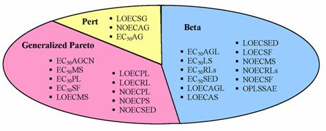
Figure 5. Classification of activities and total energy according with maximum likelihood criterion on correlation coefficients for quantitative structure-activity/property relationships
The analysis of Table 10 reveals the following:
§ Just one misclassification is observed for Chi-Squared statistic. This result suggests that Chi-Squared statistic should be used to partition activities of studied ordnance compounds in relation to the correlation coefficient distribution laws. This fact could probably be explained by the fact that the Chi-Squared statistic is exposed only to type I errors [50].
§ Kolmogorov-Smirnov statistic misclassified the maximum likelihood 12 times, which suggests that it is not the proper statistic for partition activities of studied ordnance compounds.
§ The Agr/Param ratio proved able to discriminate with a high power using minimum of parameters according to principle of Occam's razor [51] (parsimony – recommends to select the hypothesis that makes the fewer assumptions when more hypotheses are probably equal [18,52].
The analysis of Figure 5 identified that almost 48% of correlation coefficients associated to simple linear regression models proved fit Beta distribution when MDFV descriptors were used to explain ordnance compounds toxicities and total energy. Moreover, 40% proved fit Generalized Pareto distribution and 12% fit Pert distribution.
The pattern distribution laws on correlation coefficient may classify the structure-activity relationships. Identification of a certain distribution law of correlation coefficient allows calculation of the probability to obtain a structure-activity relationship with a certain (desired) correlation coefficient. For example, the probability to obtain a relationship with correlation above 0.99 for LOEC(SG) is 5.46‰ (1-CDFPert(x; 0.73539, 0.70693, 1.1102) - from Pert distribution law; data in Supplementary material).
The distribution law of correlation coefficients in simple linear regression on quantitative structure-activity/property relationships was successfully analyzed and certain pathways were identified. But, what does this study add to the field? Generally, there is no technique able to provide a best QSAR model other than selection of those descriptors from the pool of descriptors in such way to obtain a determination coefficient as far as possible to the right tail of the distribution of correlation coefficients from all possible QSAR models who to assure both internal and external validity. Valid results applied on investigated data were obtained but as expected our study has its limitations. Neither internal nor external validation of the identified QSAR/QSPR models was conducted since it was not the aim of present research; but just valid regression models were included in this analysis. The analysis of correlation coefficient distribution on QSAR/QSPR internally valid models could identify the differences between distribution laws of correlation coefficient and leave-one-out correlation coefficient, and this is a task that could be investigated. The results of our study can certainly be applied on the investigated sample of compounds and on the studied toxicities/properties. Further investigations will be carried out in our laboratory in order to assess whether the identified pathway of joined PDFs associated to the correlation coefficients of QSAR/QSPR models fit any set of compounds and any activities/properties. The toxicity investigated in this research is the main read-out for the ordnance compounds and the causes could be multiples and the identification of the linear model is used just to express quantitatively the link between ordnance compounds structure and their toxicity not to assess the toxicity pathways. This is what is knows as applicability domain of a quantitative structure-activity relationship. Thus, it is likely that a QSAR model with one descriptor to take into account one factor able to explain the link between compound structure and its toxicity, while a QSAR model with 2 descriptors to take into account two factors (able to explain the observed toxicity). Ongoing studies in our laboratory aim to demonstrate whether the results of this study reflect the distribution of both correlation coefficient and leave-one-out correlation coefficient in QSARs.
Conclusions
The correlation coefficients of QSAR/QSPR models obtained on ordnance compounds proved not fit the same distribution law.
Both number of adapted descriptors (that can be used in regressions) and number of probable descriptors (that should be used in regression) fit Fisher-Tippett distribution. Even if 1 out of 6 descriptors qualifies to be used in regression, only 1 out of 9 provides a clear distinction from the random effect.
Three particular distribution laws were able to cover the whole space of the general distribution of the correlation coefficient on structure-activity relationships: Pert, Generalized Pareto and Beta distribution. Therefore, it is likely that depending on the investigated activity, the obtained correlation coefficient on a structure-activity relationship to be drawn from one of these distributions. This fact may become a useful tool for defining the applicability domain of a quantitative structure-activity relationship in probabilistic terms.
Chi-Squared statistic proved the proper criterion for the partition of biological activities and total energy according to the distribution law of correlation coefficients obtained in simple linear regressions using MDFV descriptors.
Acknowledgements
This paper is dedicated to Professor Ante Graovac on his 65th birthday.
The study was supported by POSDRU/89/1.5/S/62371 through a postdoctoral fellowship for L. Jäntschi. The funding source had no role in study design, data collection, analysis and or interpretation of data, in the writing of the report or in the decision to submit the article for publication.
References
1. Fisher R.A., Frequency distribution of the values of the correlation coefficient in samples from an indefinitely large population, Biometrika, 1915, 10, p. 507-21.
2. Zimmerman D.W., Zumbo B.D., Williams R.H., Bias in Estimation and Hypothesis Testing of Correlation, Psicológica, 24, 2003, p. 133-58.
3. Olkin I., Pratt J.W., Unbiased estimation of certain correlation coefficients, Annals of Mathematical Statistics, 1958, 29, p. 201-11.
4. Pearson E.S., Adyanthāya N.K., The distribution of frequency constants in small samples from non-normal symmetrical and skew populations, Biometrika, 1929, 21, p. 259-86.
5. Rider P.R., On the distribution of the correlation coefficient in small samples, Biometrika, 1932, 24, p. 382-403.
6. Gayen A.K., The Frequency Distribution of the Product-Moment Correlation Coefficient in Random Samples of any Size Drawn from Non-Normal Universes, Biometrika, 1951, 38, p. 219-247.
7. Tasker G.D., Approximate sampling distribution of the serial correlation coefficient for small samples, Water Resources Research, 1983, 19, p. 579-582.
8. **EC2001. European Commission, Strategy for a Future Chemicals Policy. Brussels, Belgium: Commission of the European Communities. (2001). http://www.isopa.org/isopa/uploads/Documents/documents/White%20Paper.pdf (Accessed June 2010).
9. Ferreira J.E.V., Figueiredo A.F., Barbosa J.P., Cristino M.G.G., Macedo W.J.C., Silva O.P.P., Malheiros B.V., Serra R.T.A., Ciriaco-Pinheiro J., A study of new antimalarial artemisinins through molecular modeling and multivariate analysis, Journal of the Serbian Chemical Society, 2010, 75, p. 1533-48.
10. Hansch C., Maloney P.P., Fujita T., Muir R.M., Correlation of Biological Activity of Phenoxyacetic Acids with Hammett Substituent Constants and Partition Coefficients, Nature, 1962, 194, p. 178-180.
11. Lagunin A.A., Zakharov A.V., Filimonov D.A., Poroikov V.V., A new approach to QSAR modelling of acute toxicity, SAR and QSAR in Environmental Research, 2007, 18, p. 285-98.
12. Borota A., Mracec M., Gruia A., Rad-Curpan R., Ostopovici-Halip L., Mracec M., A QSAR study using MTD method and Dragon descriptors for a series of selective ligands of alpha C-2 adrenoceptor, European Journal of Medicinal Chemistry, 2011, 46, p. 877-84.
13. Mercado J., Gomez H., Vivas-Reyes R., Comparative molecular field analysis and comparative molecular similarity indices analysis studies of alpha-ketothiazole arginine analogues inhibitors of coagulation factor XIa, New Journal of Chemistry, 2011, 35, p. 820-32.
14. Marrero-Ponce Y., Martinez E.R., Casanola-Martin G.M., Perez-Gimenez F., Diaz Y.E., Garcia-Domenech R., Brogues J.E.R., Bond-Extended Stochastic and Nonstochastic Bilinear Indices. I. QSPR/QSAR Applications to the Description of Properties/Activities of Small-Medium Size Organic Compounds, International Journal of Quantum Chemistry, 2011, 111, p. 8-34.
15. Acharya C., Coop A., Polli J.E., MacKerell A.D., Recent Advances in Ligand-Based Drug Design: Relevance and Utility of the Conformationally Sampled Pharmacophore Approach, Current Computer-Aided Drug Design, 2011, 7, p. 10-22.
16. Munei Y., Shimamoto K., Harada M., Yoshida T., Chuman H., Correlation analyses on binding affinity of substituted benzenesulfonamides with carbonic anhydrase using ab initio MO calculations on their complex structures (II), Bioorganic & Medicinal Chemistry Letters, 2011, 21, 141-4.
17. Jäntschi L., Bolboacă S.D., Results from the use of molecular descriptors family on structure property/activity relationships, International Journal of Molecular Sciences, 2007, 8, p. 189-203.
18. Jäntschi L., Genetic Algorithms and their Application, PhD Thesis in Horticulture, completed at University of Agricultural Sciences and Veterinary Medicine Cluj-Napoca, (PhD Advisor: Prof. Dr. Sestraş RE), 2010, p. 38.
19. Bolboacă S.D., Jäntschi L., Comparison of QSAR Performances on Carboquinone Derivatives, TheScientificWorldJOURNAL, 2009, 9, p. 1148-66.
20. Hoffmann R., An Extended Hückel Theory. I. Hydrocarbons, Journal of Chemical Physics, 1963, 39, p. 1397-412.
21. Bolboacă S.D., Marta M.M., Jäntschi L., Binding affinity of triphenyl acrylonitriles to estrogen receptors: quantitative structure-activity relationships, Folia Medica, 2010, 52, p. 37-45.
22. Jäntschi L., Bolboacă S.D., Furdui C.M., Characteristic and counting polynomials: modelling nonane isomers properties, Molecular Simulation, 2009, 35, p. 220-7.
23. Jäntschi L., Bolboacă S.D., Modeling the octanol-water partition coefficient of substituted phenols by the use of structure information, International Journal of Quantum Chemistry, 2007, 107, p. 1736-44.
24. Bolboacă S.D., Jäntschi L., A Structural Informatics Study on Collagen, Chemical Biology & Drug Design, 2008, 71, p. 173-9.
25. Zhang Y.M., Yang X.S., Sun C., Wang L.S.,. Quantitative structure-activity relationship of compounds binding to estrogen receptor beta based on heuristic method, Science China-Chemistry, 2011, 54, p. 237-43.
26. Jäntschi L., Bolboacă S.D., Sestraş R.E., A Study of Genetic Algorithm Evolution on the Lipophilicity of Polychlorinated Biphenyls, Chemistry & Biodiversity, 2010, 7, p. 1978-89.
27. Jäntschi L., Bolboacă S.D., Sestraş R.E., Meta-heuristics on quantitative structure-activity relationships: study on polychlorinated biphenyls. Journal of Molecular Modeling, 2010, 16, p. 377-86.
28. Gupta V.K., Khani H., Ahmadi-Roudi B., Mirakhorli S., Fereyduni E., Agarwal S., Prediction of capillary gas chromatographic retention times of fatty acid methyl esters in human blood using MLR, PLS and back-propagation artificial neural networks, Talanta, 2011, 83, p. 1014-22.
29. Fjell C.D., Jenssen H., Chng W.A., Hancock R.E.W., Cherkasov A., Optimization of Antibacterial Peptides by Genetic Algorithms and Cheminformatics, Chemical Biology & Drug Design, 2011, 77, p. 48-56.
30. Lagunin A., Zakharov A., Filimonov D., Poroikov V., QSAR Modelling of Rat Acute Toxicity on the Basis of PASS Prediction, Molecular Informatics, 2011, 30, p. 241-50.
31. Le-Thi-Thu H., Cardoso G.C., Casanola-Martin G.M., Marrero-Ponce Y., Puris A., Torrens F., Rescigno A., Abad C., QSAR models for tyrosinase inhibitory activity description applying modern statistical classification techniques: A comparative study, Chemometrics and Intelligent Laboratory Systems, 2010, 104, p. 249-59.
32. Oliveira K.M.G., Takahata Y., QSAR modeling of nucleosides against amastigotes of Leishmania donovani using logistic regression and classification tree, QSAR & Combinatorial Science, 2008, 27, p. 1020-7.
33. Hattotuwagama C.K., Doytchinova I.A., Guan P., Flower D.R., In silico QSAR-based predictions of class I and class II MHC epitopes, In: Immunoinformatics, Editors, C. Schoenbach, S. Ranganathan, V. Brusic, Sprinder Science+Business Media, LLC, New York, 2007, pp. 63-89.
34. Rodgers S.L., Davis A.M., Tomkinson N.P., van de Waterbeemd H., Predictivity of Simulated ADME AutoQSAR Models over Time, Molecular Informatics, 2011, 30, p. 256-66.
35. Ferreira L.G., Leitao A., Montanari C.A., Andricopulo A.D., Comparative Molecular Field Analysis of a Series of Inhibitors of HIV-1 Protease, Medicinal Chemistry, 2011, 7, p. 71-9.
36. Hemmateenejad B., Yousefinejad S., Mehdipour A.R., Novel amino acids indices based on quantum topological molecular similarity and their application to QSAR study of peptides, Amino Acids, 2011, 40, p. 1169-83.
37. Luo X.C., Krumrine J.R., Shenvi A.B., Pierson M.E., Bernstein P.R., Calculation and application of activity discriminants in lead optimization, Journal of Molecular Graphics & Modelling, 2010, 29, p. 372-81.
38. Golbraikh A., Shen M., Xiao Z., Xiao Y.-D., Lee K.-H., Tropsha A., Rational selection of training and test sets for the development of validated QSAR models, Journal of Computer-Aided Molecular Design, 2003, 17, p. 241-53.
39. *** Development of marine sediment toxicity for ordnance compounds and toxicity identification evaluation studies at select naval facilities. [Online], 2000, Available at: http://web.ead.anl.gov/ecorisk/issue/pdf/tox_marine_sed.pdf. Accessed March 10, 2010.
40. Sacks J., Ylvisaker D., Designs for Regression Problems with Correlated Errors III, Annals of Mathematical Statistics, 1970, 41, p. 2057-74.
41. Jarque C.M., Bera A.K., Efficient tests for normality, homoscedasticity and serial independence of regression residuals: Monte Carlo evidence, Economics Letters, 1981, 7, p. 313-18.
42. Dewar M.J.S., Zoebisch E.G., Healy E.F., Stewart J.J.P., AM1: A New General Purpose Quantum Mechanical Molecular Model, Journal of the American Chemical Society, 1985, 107, p. 3902-9.
43. Jäntschi L., Computer Assisted Geometry Optimization for in silico Modeling, Applied Medical Informatics, 2011, 29(3), p. 11-8.
44. Kendall M., A New Measure of Rank Correlation, Biometrika, 1938, 30, p. 81-9.
45. Kolmogorov A., Confidence Limits for an Unknown Distribution Function, The Annals of Mathematical Statistics, 1941, 12, p. 461-3.
46. Anderson T.W., Darling D.A., Asymptotic theory of certain "goodness-of-fit" criteria based on stochastic processes, Annals of Mathematical Statistics, 1952, 23, p. 193-212.
47. Pearson K., On the criterion that a given system of deviations from the probable in the case of a correlated system of variables is such that it can be reasonably supposed to have arisen from random sampling, Philosophical Magazine, 1900, 50, p. 157-75.
48. Fisher R.A., Combining independent tests of significance, American Statistician, 1948, 2, p. 30.
49. Fisher R.A., Tippett L.H.C., Limiting forms of the frequency distribution of the largest and smallest member of a sample, Proceedings of the Cambridge Philosophical Society, 1928, 24, p. 180-90.
50. Young R.L., Weinberg J., Vieira V., Ozonoff A., Webster T.F., Generalized Additive Models and Inflated Type I Error Rates of Smoother Significance Tests, Computational Statistics & Data Analysis, 2011, 55, p. 366-74.
51. *** "Ockham’s razor". Encyclopædia Britannica. Encyclopædia Britannica Online. [Online] Available at: http://www.britannica.com/EBchecked/topic/424706/Ockhams-razor. Accessed on 3 June 2010.
52. Sober E., Parsimony in Systematics: Philosophical Issues, Annual Review of Ecology and Systematics, 1983, 14, p. 335-57.