Resistance to Crack Propagation of Algerian Wood

Resistance to Crack Propagation of Algerian Wood

Salim KENNOUCHE ¹, Abdelatif ZERIZER ¹, Rémy MARCHAL ², Abdelhamid AKNOUCHE ¹, and Abdelhakim DAOUI ¹

¹EMMF, UR-MPE, FSI, UMBB, 35000 Independence Avenue of Boumerdes, Algeria

²CER ENSAM, Rue Porte de Paris, Cluny, France

E-mails: kennouchesalim@yahoo.fr, zerizer_ab@yahoo.fr, Marchal.remy@cluny.ensam.fr, h.aknouche@yahoo.fr, daouiabdelhakim@yahoo.fr.

^*Corresponding author: Phone 00213 550752567

Abstract

Wood is the most building materials widely used since prehistory for the construction of houses, tools, weapons. Accidents occurring during the use of materials caused by different defaults, as: knots, resin pockets, cracks. These various defaults and others are the starting point of the principle of crack mechanics. Our present work focuses on determining the resistance to crack propagation of three types of Algerians wood, (Aleppo pine, eucalyptus and oak), by calculating the energy release rate G (mode I). The estimation of factor G allows the possibility of fracture propagation.

Keywords

Wood; Fracture Mechanics; Energy Release Rate.

Introduction

Wood is a building materials which has a technological impact, the economic one is sometimes more important than some other materials [1]. For these reasons, the wooden building user and designer seek to better understand the mechanical properties of the material to improve performance and reliability of their achievement, while seeking to reduce costs.

Incidents that occur during the use of materials are due to; presence of cracks, then a boot with propagation to failure, which constitutes the basis of fractures mechanics.

Recall the Fracture Mechanics

Brittle fracture, in the absence of significant plastic deformation (mechanical linear fracture) [2].

Ductile fracture, in the presence of significant plastic deformation (nonlinear mechanics of fracture). In this case, according to the size of the plastic zone at the crack tip, it distinguishes the case of confined plasticity, of the extent of plasticity [2].

Modes of rupture: The cracking occurs by the irreversible separation of a continuous medium into two parts, called lips of the crack, which introduces a discontinuity in the path of travel.The possible movements of the lips of each crack are combinations of three independent modes that the figure 1 mention, according to [3].

Figure 1. Mode of rupture, Mode I: Opening (or cleavage) mode II shear plane, mode III antiplane shear [4]

Concentration coefficients k and intensity factor K. Figure 2 defines a coordinate system at the crack tip and the constraints associated with a small volume element, according to Triboulot [1]. In this system, the stresses at the crack tip are determined using the following relationships according to Engerand [5]:

where σx: Stress along x; σy: Stress along y; t xy: Shear Stress by xy; KI: stress factor intensity in mode I, KI: factor intensity of constraint in mode II.

Figure 2. Coordinate system at the tip of the crack

It is important not to confuse the coefficient of stress concentration k which gives only local information at the very point of the crack and the stress factor intensity K, which describes all the spatial singularity of the field constraint. If k is dimensionless, K is the product of constraint by the square root of length

[k] = σ [T] 1 / 2 and is measured in MPa.

The passage to the limit to define a crack as the limit of an elliptical hole completely flattened naturally leads to a relationship between two quantities, the length involved in K being related to the size “a” of the default by Irwin relationship

r→0

where, σm being forced into the elliptic crack tip and r its radius of curvature.

For c flat elliptical crack of length 2c in an infinite plate (in practice to large-sized c) subject to tension σ, σm = kσ where k = 2, the passage to the limit leads KI = σ, as the figure 3 mention.

Figure 3. Stress factor intensity

The energy release rate: G, the energy release rate represents the energy required to advance the crack of a unit length. It corresponds to the decrease in the total potential energy Wp to move from an initial configuration with length “a” of crack, to another where the crack propagated by a length da.

where W_e represents the elastic strain energy, w_ext the potential energy of the external forces f, and ∂ A the increment of surface corresponding to the extension of the crack.

Using the stress field in the singular zone and the law of linear elastic behavior, it is possible to link the release energy rate to stress factors intensity, as the equations, according to Hakim [6].

where E is Young's modulus and ν Poisson's ratio.

So as cited in bibliography [7], G expresses the rate of energy change corresponding to a small crack growth da. Analytical form, we write:

KI2 = G (k + 1) / μ 8 with k = 3 - 4υ in plane strain and k = (3 - υ) / (1 - υ) in plane stress: In plane stress: G = KI2 / E; Plane strain: G = (1 - υ2) KI2 / E.

On the curve force / displacement following cons, OA corresponds to a crack length a, and OB at a crack length a + δa. G represents the area situated in the triangle OAB for a test at the burden or the triangle OAC for a driving the displacement imposed.

The figure 4 and 5 present the graphical method of calculating the energy release rate and the J determination by graphical method.

Figure 4. Method of calculating the energy release rate G

Figure 5. Determination of J by the method of complaisance

Determination of energy release rate G: To make a calculation, a graphic tool is called to calculate the area under the force- displacement curves obtained for cut specimens, with a₁ = 4 mm and a₂ = 8 mm, the area between the two curves corresponds to energy in joules it takes to move the crack a₁ = 4 mm and a₂ = 8 mm.

The experimental results, values of the energy release rate G until the break and elastic limit are represented in the following table.

Experimental Approach

Materials: Zeen oak, Aleppo pine and eucalyptus are the three species used in this work, whose provenance is the unit of trans-wood of Bejaia (Algeria) for Alep pine, and the regional station the National Research Institute of Forestry (INRF) of Azazga in the wilaya of Tizi Ouzou.

Preparation of test specimens: The raw material is put into water to prevent its decay, the last one is taken out, sawn, planed and put into standard specimens (20 × 20 × 340), intended for mechanical testing, and specimen (20 × 20 × 20) for physical testing.

$F:\photos vidéo memoire\photos memoir\photos labo le 19 juin 09\Photo 047.jpg$

Figure 6. Specimen test

Preparation of cuts: After preparing the Specimens test was conducted to prepare cuts deep a₁ = 4mm, a₂= 8 mm which will also be sought in three-point bending.

Figure 7. Specimens cut (a₁ = 4 mm, a₂ = 8 mm)

Physical-Mechanical Characterization

Physical Test (Standard NF B 51-152): The specimens (20 × 20 × 20) are characterized physically, which we determined the densities, and swelling and withdrawal under the three main directions, longitudinal, radial and tangential.

Results of physical characteristics: The results of densities of the three species studied are presented in the table 1.

Table 1. Results of the physical characteristics of the three species studied at 12% humidity

Properties Wood	Mv (g/cm³)	Sw_L (%)	Sw_R(%)	Sw_T (%)	Wit_L (%)	Wit_R(%)	Wit_T (%)
Alep pin	0.57	0.79	1.65	2.62	0.29	4.84	5.20
Zeen oak sapwood	0.80	0.43	3.80	3.90	1.48	8.13	6.74
Zeen oak heatwood	0.78	5.14	0.76	3.26	2.32	8.21	7.89
Eucalytus sapwood	0.65	2.69	9.16	11.33	1.05	9.75	11.96
Ecalyptus heartwood	0.62	1.18	2.91	7.08	0.39	5.80	9.21
Sw_L .R.T: swelling in longitudinal. radial and tangential direction. Ret_L.R.T: Withdrawal in longitudinal. radial and tangential direction

Mechanical Testing (Standard NA.604/1990)

Mechanical tests are realised using a Zwick universal machine. type Z010 with the software testXpert v12.0. and with a force transducer 10KN. The driving and the acquisition are done by computer. Bending at least five specimens are sought for each species from the two areas of sampling. sapwood and heartwood timber. as showing in figure 10.

Figure 10. Three-point bending test

Results and Discussion

The figures 11-15 present the force-displacement curves obtained by three point bending test on the three wood types of samples (not cat. cat at 4 mm and 8 mm).


*Figure 11.* Specemeen Alep pine wood. not cut. cut a₁ = 4 mm and a₂ = 8 mm	*Figure 12.* Cases of wood zeen oak sapwood. not cut. cut a₁ = 4 mm and a₂ = 8 mm

*Figure 13*. Cases of wood zeen oak heartwood. not cut. cut a₁ = 4 mm. a₂ = 8mm	*Figure 14.* Cases of eucalyptus woodsap. not cut . cut a₁ = 4 mm and a₂ = 8 mm

*Figure 15.* Cases of eucalyptus wood heartwood not cut. cut a₁ = 4 mm. a₂ = 8 mm

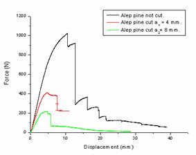
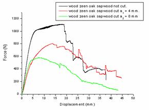
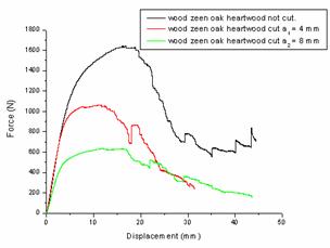
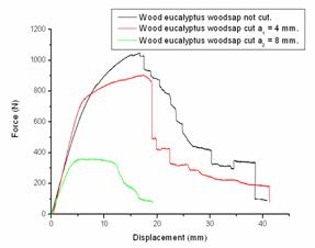
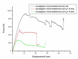
The results obtained show that the rupture strength decreases by increasing the depth of cut. This is explained by the decrease of micro fibrils involved in the mechanical strength given the presence of the cut.

This amount is divided by the surface of the crack ligament. which gives the energy release rate (G) (J/m²).

Calculation of energy release rate G: We recall that the values of the rate of energy release G. represented in the following table were calculated from force-displacement curves. it’s useful that the approach used is based on the graphical procedure using numerical calculation software.

Numerical Calculation of the Rate of Energy G

Digital Approach:

The step is taken the following steps are sited according to [8]:

§ Creation of points in two dimensions that provide the backbone of the piece;

§ Creating lines connecting points;

§ Creation of the surface of the piece;

§ Choice of the material model (elastic orthotropic) that it is introducing the elastic module of the material obtained experimentally;

§ Meshing the surface of the piece;

§ Creation of support and introduction of force. one way to achieve the three-point bending;

§ Start the calculation;

§ Extraction of the values of displacements of two nodes closest to the tip of the crack; noted uy (m) and the value of r = (x2 - xi) or x2 is the depth of the crack and xi is the nodal abscissa. As <uy> = 2uy. Finally the calculation of KI by following formula according to [9]:

where E = Young modulus; υ = Poisson's ratio; r = node coordinates; u_y= nodal displacement.
KI and G are related by the following formula: G = K²/E_L

Extrapolating the displacement obtained by EF:

We have:

where u_y is the nodal displacement.

Figure 16. Representation of nodes with finite element

Figure 17. Representation. (left-hand figure) crack tip (right-hand graph) the two nodes closest to the crack tip by digital tools

Figure 18. Structure distorted before and after load application


Along X	Along Y

Figure 19. Distribution of stress. along X. Y

After building the model, the numerical tool allows us to retrieve the values of the abscissas of the two nodes closest to the crack tip and the nodal displacements. The values of the coefficient of stress concentration are obtained, which are squared and divided by Young's modulus, and we obtain values of energy release rate G. which are given in the table 2.

Table 2. Numerical values of the energy release rate G species studied

Wood type	G (J/m²)
Alep pine	0.23
Zeen oak sapwood	1.28
Zeen oak heartwood	0.84
Eucalyptus sap	28.11
Eucalyptus heartwood	7.89

Comparative study of two methods: The results obtained by experimental and numerical calculations are presented are presented in the table 3.

Table 3. Comparison between the values of the energy release rate G obtained experimentally and numerically

Value of G (KJ/m2) Wood type	G (KJ/m²) Yield Stress	G (KJ/m²) obtained by numerical tool.	G bibliography
Alep pine	0.72	0.23	Between (0.3-6.2) J/m² in the work of TRIBULOT. and up to 80 J/m2.
Zeen oak sapwood	4.78	1.28
Zeen oak heartwood	4.58	0.84
Eucalyptus sapwood	13.28	28.11
Eucalyptus heartwood	1.33	7.89

Interpretation of the results: In the numerical calculation of the stress coefficient concentration for the different species studied, that presented in table 3, we obtained comparable results to those found in the literature. We can list the values of energy release rate obtained by TRIBOULOT and PLUVINAGE, in their work on determining the energy release rate G. which lie between (0.3 and 6.2) KJ/m² in our work we found values between 1.58 and 5.35 KJ/m² except the cases of specimens of oak zeen and the Eucalyptus from sapwood, are from 12.15 KJ/m². 18.44 KJ/m² respectively. This will induces that when comparing the results we can just decide on the size of these last ones, given the marked difference in testing protocols (conditions. nature of the material. specimen geometry).

Conclusion

In our study, we determined the energy release rate, three species of Algerian wood with a reliable experimental approach. since the results obtained are comparable to values found in literature (TRIBOULOT and PLUVINAGE).

The validation of the results by a numerical calculation, allowed us. also to find values close to that obtained experimentally in the elastic range.

References

1. Triboulot P., Jodin P., Pluvinage G., Mesure des facteurs d’intensité de contrainte critiques et des taux de restitution d’énergie dans le bois sur éprouvettes entaillées. laboratoire de Fiabilité mécanique Faculté des Sciences. Université de Metz lie du Saulcy. F 57000 Metz. Ann. Sci. Forest, 1982, 39(1), p. 63-76.

2. Dias de Moraes P., Influence de la température sur les assemblages bois. Université Henri Poincaré Nancy 1 thèse doctorale, p. 46-59, 2003.

3. K. Lakhdar. Adesifs et thechnique de collage: caractérisation de l’adhérence. Université M’Hamed Bougara de Boumerdès.Thèse de magistère, 34 p., 2006.

4. Wood handbook. Wood as an engineering material. United States department of agriculture, forest service, forest products laboratory. 1999, p. 35-39.

5. Engerand J.-L., Mécanique de la rupture. Techniques de l’Ingénieur. traité Génie Mécanique B 5 060, 1990.

6. Hakim Naceur. Rappel de cours mécanique linéaire élastique de la rupture. Université de Valencienne, 2009, p. 5-9.

7. Help logiciel de simulation ansys version 11 (28/02/2010).

8. Jeane Clande. Mécanique du solide et des matériaux (élasticité. plasticité. rupture) Laboratoire PMMH. ESPCI. 10 rue Vauquelin. 75005 Paris, 2003, p. 38-45.

9. Moustapha C., Youcef G., Méthodes de dimensionnement critères de tenue mécanique en fatigue Travaux Pratiques. INRA. UR 1268 Biopolymères. Interaction et Assemblages, 2004, p. 1-6.