A Hybrid Harmony Search Algorithm Approach for Optimal Power Flow
Mimoun YOUNES1 and Fouad KHODJA2
Faculty
of Engineering Sciences,
E-mails: 1 younesmi@yahoo.fr; 2 khodjafouad@gmail.com
* Corresponding author: Phone: (213) 7 84 47 57. ; Fax: (213) 48 42 09 12.
Abstract
Optimal Power Flow (OPF) is one of the main functions of Power system operation. It determines the optimal settings of generating units, bus voltage, transformer tap and shunt elements in Power System with the objective of minimizing total production costs or losses while the system is operating within its security limits. The aim of this paper is to propose a novel methodology (BCGAs-HSA) that solves OPF including both active and reactive power dispatch It is based on combining the binary-coded genetic algorithm (BCGAs) and the harmony search algorithm (HSA) to determine the optimal global solution. This method was tested on the modified IEEE 30 bus test system. The results obtained by this method are compared with those obtained with BCGAs or HSA separately. The results show that the BCGAs-HSA approach can converge to the optimum solution with accuracy compared to those reported recently in the literature.
Keywords
Genetic Algorithm; Harmony search algorithm; Optimal Power Flow (OPF); Optimization; Hybridization.
Introduction
Optimal Power Flow (OPF) [1] is a nonlinear programming problem, it is used to determine optimal outputs of generators, bus voltage and transformer tap setting in power system with an objective to minimize total production costs while the system is operating within its security limits. Since OPF was introduced in 1968, several methods have been employed to solve this problem, e.g. Gradient base [2], Linear programming method [3] and Quadratic programming [4]. However all of these methods suffer from three main problems. Firstly, they may not be able to provide optimal solution and usually getting stuck at a local optimal. Secondly, all these methods are based on assumption of continuity and differentiability of objective function which does not actually exist in a practical system. Finally, all these methods cannot be applied with discrete variables, which are transformer taps. The binary-coded genetic algorithm (BCGAs) approach is an appropriate method that we could use.
Indeed
its algorithm is well suited for the resolution of our problem which eliminates
the above drawbacks, BCGAs invented by
BCGAs operate on a population of candidate solutions encoded to finite bit string called chromosome.
In order to obtain optimality, each chromosome exchanges information by using operators borrowed from natural genetic to produce the better solution.
BCGAs differ from other optimization and search procedures in four ways [6]:
§ BCGAs work with a coding of the parameter set, not the parameters themselves. Therefore GAs can easily handle the integer or discrete variables.
§ BCGAs search from a population of points, not a single point. Therefore BCGAs can provide globally optimal solutions.
§ BCGAs use only objective function information, not derivatives or other auxiliary knowledge. Therefore BCGAs can deal with the non-smooth, non-continuous and non-differentiable functions which exist actually in a practical optimization problem.
§ BCGAs use probabilistic transition rules, not deterministic rules although BCGAs seem to be a good method to solve optimization problem, sometimes the solution obtained from BCGAs is only a near global optimum solution. Therefore this paper employs BFGS applied with BCGAs to obtain the global solution. Basically, this method can be divided into two parts. The first part employs BCGAs to obtain a near global solution, while the other part employs HS to reactivate the research process and avoid premature convergence. This method was tested on the modified IEEE-30 bus test system. The result of the study of this method is compared with those obtained from BCGAs (binary-coded genetic algorithm) or HSA separately.
Optimal Power Flow Formulation
The OPF
problem is to find the optimal combination of power generation that minimizes
the total cost while satisfying the total demand. The cost function of OPF
problem is defined as follows [4]:
![]() (1)
(1)
In Eq. (1), the generation cost function ![]() in
US$/h is usually expressed as a quadratic polynomial [8]
in
US$/h is usually expressed as a quadratic polynomial [8]
![]() (2)
(2)
where: ![]() = Total production cost ($/h);
= Total production cost ($/h); ![]() = The cost of the ith
generator in $/h;
= The cost of the ith
generator in $/h; ![]() =
The power output of generator i
in MW;
=
The power output of generator i
in MW; ![]() the
cost coefficients of the ith
generator.
the
cost coefficients of the ith
generator.
In minimizing the cost, the equality constraint (power balance) and
inequality constraint (power limits) should be satisfied.
![]() (3)
(3)
where: ![]() = Active power load at bus
j;
= Active power load at bus
j; ![]() =
Active power generation at bus i;
=
Active power generation at bus i; ![]() =
Real losses.
=
Real losses.
The generation capacity of each generator has some limits and it can be
expressed as
![]() (4)
(4)
where: ![]() = Lower and upper limit of
active power generation at bus i; N =
number of bus; ND = number of load buses; NG = number of
generator.
= Lower and upper limit of
active power generation at bus i; N =
number of bus; ND = number of load buses; NG = number of
generator.
The proposed method guarantees the near optimal solution and remarkably reduces the computation time.
The transmission loss can be represented by the B-coefficient method as
![]() (5)
(5)
where ![]() is the
transmission loss coefficient,
is the
transmission loss coefficient, ![]() the power
generation of ith and jth
units. The B-coefficients are found through the Z-bus calculation
technique.
the power
generation of ith and jth
units. The B-coefficients are found through the Z-bus calculation
technique.
Genetic Algorithm
For
the application of the genetic algorithm, we use the method of penalty [7]:
![]() , (i=0…
m) are the constraints of the inequality type,
, (i=0…
m) are the constraints of the inequality type,
![]() , (j=0… n) are
the constraints of the equality type,
, (j=0… n) are
the constraints of the equality type,
By transforming the problem into a function of penalty, we obtain:
![]() (6)
(6)
where: ![]() is the coefficient
of penalization the functions of penalty
is the coefficient
of penalization the functions of penalty ![]() et
et ![]() are determined by three methods of penalty:
are determined by three methods of penalty:
§
Method of
external penalty:
![]() and
and
![]()
The function
of penalty to be solved becomes:
![]() (7)
(7)
§ Method of interior penalty:
In this
case, only the constraints of inequality are taken into account and are defined
as follows:
![]() the function to be
minimized will be:
the function to be
minimized will be:
 (8)
(8)
§ Method of penalty mixed:
It acts in this method of a combination of both premieres
![]() and
and
![]()
The function
to be minimized will be:
 (9)
(9)
Representation
It turns out that there is no rigorous definition of "genetic algorithm" accepted by all in the evolutionary-computation community that differentiates genetic algorithm (Gas) from other evolutionary computation methods [8].
However, it can be said that most methods called "GAs" have at least the following elements in common:
Populations of chromosomes, selection according to fitness, crossover to produce new offspring are random.
The chromosomes in a GAs population typically take the form of bit strings. Each locus in the chromosome has two possible alleles: 0 and 1. Each chromosome can be thought of as a point in the search space of candidate solutions. The GAs processes populations of chromosomes, successively replacing one such population with another. The GAs most often requires a fitness function that assigns a score (fitness) to each chromosome in the current population. The fitness of a chromosome depends on how well that chromosome solves the problem at hand.
GAs Operators
The simplest form of genetic algorithm involves three types of operators: selection, crossover (single point), and mutation [5].
Selection
This operator selects chromosomes in the population for reproduction. The fitter the chromosome, the more times it is likely to be selected to reproduce [6].
Crossover
This operator randomly chooses a locus and exchanges the subsequences before and after that locus between two chromosomes to create two offspring. For example, the strings 10000100 and 11111111 could be crossed over after the third locus in each to produce the two offspring 10011111 and 11100100. The crossover operator roughly mimics biological recombination between two single-chromosome (haploid) organisms.
Mutation
This operator randomly flips some of the bits in a chromosome [11]. For example, the string 00000100 might be mutated in its second position to yield 01000100. Mutation can occur at each bit position in a string with some probability, usually very small (e.g., 0.001).
A binary-Coded Genetic Algorithm (BCGAs)
Given a clearly defined problem to be solved and a bit string representation for candidate solutions, a simple BCGAs [7] works as follows:
1. Start with a randomly generated population of n l-bit chromosomes (candidate solutions to a problem).
2. Calculate the fitness ƒ(x) of each chromosome x in the population.
3. Repeat the following steps until n offspring have been created:
§ Select a pair of parent chromosomes from the current population, the probability of selection being an increasing function of fitness. Selection is done "with replacement," meaning that the same chromosome can be selected more than once to become a parent.
With probability pc (the "crossover probability" or "crossover rate"), cross over the pair at a randomly chosen point (chosen with uniform probability) to form two offspring. If no crossover takes place, form two offspring that are exact copies of
§ Their respective parents. (Note that here the crossover rate is defined to be the probability that two parents will cross over in a single point [9]. There are also "multi-point crossover" versions of the BCGAs in which the crossover rate for a pair of parents is the number of points at which a crossover takes place.)
§ Mutate the two offspring at each locus with probability pm (the mutation probability or mutation rate), and place the resulting chromosomes in the new population. If n is odd, one new population member can be discarded at random.
4. Replace the current population with the new population.
5. Go to step 2. Each iteration of this process is called a generation. BCGAs are typically iterated for anywhere from 50 to 500 or more generations. The entire set of generations is called a run. At the end of a run there are often one or more highly fit chromosomes in the population. Since randomness plays a large role in each run, two runs with different random-number seeds will generally produce different detailed behaviours. BCGAs researchers often report statistics (such as the best fitness found in a run and the generation at which the individual with that best fitness was discovered) averaged over many different runs of the BCGAs on the same problem (Figure 1).
The simple procedure just described is the basis for most applications of BCGAs. There are a number of details to fill in, such as the size of the population and the probabilities of crossover and mutation, and the success of the algorithm often depends greatly on these details. There are also more complicated versions of BCGAs (e.g., BCGAs that work on representations other than strings or BCGAs that have different types of crossover and mutation operators).
As a more detailed example of a simple BCGAs, suppose that l (string length) is 8, that ƒ(x) is equal to the number of ones in bit string x (an extremely simple fitness function, used here only for illustrative purposes), that n (the population size) is 4, that pc = 0.7, and that pm = 0.001. (Like the fitness function, these values of l and n were chosen for simplicity. More typical values of l and n are in the range 50–1000. The values given for pc and pm are fairly typical.) The initial (randomly generated) population might look like this:
Table 1. The initial (randomly generated) population
|
Chromosome label |
Chromosome string |
Fitness |
|
A |
00000110 |
2 |
|
B |
11101110 |
6 |
|
C |
00100000 |
1 |
|
D |
00110100 |
3 |
A common selection method in BCGAs is fitness-proportionate selection, in which the number of times an individual is expected to reproduce is equal to its fitness divided by the average of fitness in the population. (This is equivalent to what biologists call "viability selection")
A simple method of implementing fitness-proportionate selection is "roulette-wheel sampling", which is conceptually equivalent to giving each individual a slice of a circular roulette wheel equal in area to the individual's fitness. The roulette wheel is spun, the ball comes to rest on one wedge-shaped slice, and the corresponding individual is selected. In the n = 4 example above, the roulette wheel would be spun four times; the first two spins might choose chromosomes B and D to be parents, and the second two spins might choose chromosomes B and C to be parents. (The fact that A might not be selected is just the luck of the draw. If the roulette wheel were spun many times, the average results would be closer to the expected values) Once a pair of parents is selected, with probability pc they cross over to form two offspring. If they do not cross over, then the offspring are exact copies of each parent. Suppose, in the example above, that parents B and D cross over after the first bit position to form offspring E = 10110100 and F = 01101110, and parents B and C do not cross over, instead forming offspring that are exact copies of B and C. Next, each offspring is subject to mutation at each locus with probability pm. For example, suppose offspring E is mutated at the sixth locus to form E' = 10110000, offspring F and C are not mutated at all, and offspring B is mutated at the first locus to form B' = 01101110. The new population will be the following:
Table 2. The new population
|
Chromosome label |
Chromosome string |
Fitness |
|
E’ |
10110000 |
3 |
|
F |
01101110 |
5 |
|
C |
00100000 |
1 |
|
B’ |
01101110 |
5 |
Figure 1. The general structure of standard genetic algorithm
Real Genetic Algorithm (RGA)
RGA is a probabilistic search technique, which generates the initial parent vectors distributed uniformly in intervals within the limits and obtains global optimum solution over number of iterations [10].
The
implementation of RGA is given below. The initial population is generated after
satisfying the equation (5). The elements of parent vectors ![]() are
the real power outputs of generating units distributed uniformly between their
minimum and maximum limits.
are
the real power outputs of generating units distributed uniformly between their
minimum and maximum limits.
The fitness function is used to transform the cost function value into a measure of relative fitness. The cost function is given in equation (1).
The selection is based
on the cost of parent vectors ![]() with the corresponding
cost of offspring vectors
with the corresponding
cost of offspring vectors ![]() in this
population. The best vector having minimum cost, whether
parent vector
in this
population. The best vector having minimum cost, whether
parent vector ![]() or offspring vector
or offspring vector ![]() is
selected for the new parent for the next generation. A non-uniform
arithmetic crossover operator is used. After crossover is completed,
non-uniform mutation is performed. In the mutation step, a random real value
makes a random change in the mth element of
the chromosome [11]. After mutation, all constraints are checked whether
violated or not. If the solution has at least one constraint violated, a new
random real value is used for finding a new value of the m-th element of the chromosome. Then, the best solution so
far obtained in the search is retained and used in the following generation.
The RGA process repeats until the specified maximum number of generations is
reached [12]. This can be summarized briefly as shown in the flowchart of
Figure 2.
is
selected for the new parent for the next generation. A non-uniform
arithmetic crossover operator is used. After crossover is completed,
non-uniform mutation is performed. In the mutation step, a random real value
makes a random change in the mth element of
the chromosome [11]. After mutation, all constraints are checked whether
violated or not. If the solution has at least one constraint violated, a new
random real value is used for finding a new value of the m-th element of the chromosome. Then, the best solution so
far obtained in the search is retained and used in the following generation.
The RGA process repeats until the specified maximum number of generations is
reached [12]. This can be summarized briefly as shown in the flowchart of
Figure 2.
Figure 2. The general structure of Real Genetic Algorithm (RGA)
Harmony Search Algorithm (HSA)
Harmony search algorithm is a novel meta-heuristic algorithm, which has been conceptualized using the musical process of searching for a perfect state of harmony. This meta-heuristic is based on the analogy with music improvisation process where music players improvise the pitches of their instruments to obtain a better harmony. In the optimization context, each musician is replaced with a decision variable, and the possible notes in the musical instruments correspond to the possible values for the decision variables.
The harmony in music is analogous to the optimization solution vector, and the musician’s improvisations are analogous to local and global search schemes in optimization techniques.
Musical performances seek to find pleasing harmony (a perfect state) as determined by an aesthetic standard, just as the optimization process seeks to find a global solution (a perfect state) as determined by an objective function [13].
The parameters of HS method are: the harmony memory size (HMS), the harmony memory considering rate (HMCR), the pitch adjusting rate (PAR), and the number of improvisations (NI). The harmony memory is a memory location where a set of solution vectors for decision variables is stored. The parameters HMCR and PAR are used to improve the solution vector and to increase the diversity of the search process. In HS, a new harmony (i.e., a new solution vector) is generated using three rules: 1) memory consideration, 2) pitch adjustment, and 3) random selection. It is convenient to note that the creation of a new harmony is called “improvisation”. If the new solution vector (i.e., new harmony) is better than the worst one stored in HM, this new solution updates the HM. This iterative process is repeated until the given termination criterion is satisfied. Usually, the iterative steps are performed until satisfying the following criterions: either the maximum number of successive improvisations without improvement in the best function value, or until the maximum number of improvisations is satisfied [14].
This can be summarized briefly as shown in the flowchart of Figure 3.
Figure 3. Flowchart of the HSA procedure
Initialize the problem and algorithm parameters
The optimization problem is defined as follows:
Minimize f(x) subject to xi Є Xi , i=1,……., N. where f(x) is the objective function, x is the set of each decision variable (xi ); Xi is the set of the possible range of values for each design variable, that is XiL < Xi < XiU, where XiL and XiU are the lower and upper bounds for each decision variables.
The HSA parameters are also specified in this step. They are the harmony memory size (HMS) [15], or the number of solution vectors in the harmony memory; harmony memory considering rate (HMCR); bandwidth (BW); pitch adjusting rate (PAR); number of improvisations (NI) or stopping criterion and number of decision variables (N).
Initialize the Harmony Memory (HM)
The
harmony memory is a memory location where all the solution vectors (sets of
decision variables) are stored. HM matrix is filled with as many randomly
generated solution vectors as the HMS.
 (10)
(10)
Improvise a New Harmony
A
new harmony vector, ![]() , is generated based on the three
rules: (1) memory consideration, (2) pitch adjustment and (3) random selection.
, is generated based on the three
rules: (1) memory consideration, (2) pitch adjustment and (3) random selection.
Generating a new harmony is called (improvisation).
The value
of the first decision variable ![]() for the new vector can
be chosen from any value in the specified HM range
for the new vector can
be chosen from any value in the specified HM range![]() .
.
Values
of the other design variables ![]() are
chosen in the same manner.
are
chosen in the same manner.
HMCR,
which varies between 0 and 1, is the rate of choosing one value from the
historical values stored in the HM, while (1- HMCR) is the rate of randomly
selecting one value from the possible range of values.
 (11)
(11)
For
instance, a HMCR of 0.95 indicates that the HSA will choose the decision
variable value from historically [16] stored values in the HM with the 95%
probability or from the entire possible range with the 100-95% probability.
Every component of the
![]() , is examined to determine whether
it should be pitch-adjusted. This operation uses the PAR parameter, which is
the rate of pitch adjustment as follows:
, is examined to determine whether
it should be pitch-adjusted. This operation uses the PAR parameter, which is
the rate of pitch adjustment as follows:
![]() (12)
(12)
The value of (1- PAR) sets
the rate of doing nothing. If the pitch adjustment decision for x' is
Yes, x' is replaced as follows:
![]() (13)
(13)
where BW is an arbitrary distance
bandwidth for the continuous design variable and rand is a random number
between 0 and 1. In step 3, HM consideration, pitch adjustment or random
selection is applied to each variable of the
Update Harmony Memory
If
the new harmony vector, ![]() , is better than the worst harmony in
the HM, from the point of view of objective function value, the new harmony
[16] is included in the HM and the existing worst harmony is excluded from HM.
, is better than the worst harmony in
the HM, from the point of view of objective function value, the new harmony
[16] is included in the HM and the existing worst harmony is excluded from HM.
Check the Stopping Criterion
If the stopping criterion (i.e.) maximum number of improvisations is satisfied, computation is terminated. Otherwise, Step 3 and 4 are repeated.
Methodology
Traditionally, BCGAs is a stochastic optimization method which starts from multiple points to obtain a solution, but it provides only a near global solution. Similarly for HSA.
Therefore, in order to obtain a high quality solution, the two parts method, comprising both BCGAs and HSA is proposed in this paper.
In the proposed method, after the specified termination criteria for the BCGAs is reached, HSA is applied in the second part by using the solution from BCGAs as initial points to obtain a solution which is closer to the global solution at the final, This can be summarized briefly as follows:
Step 1: Read system data.
Step 2: Solve OPF problem using BCGAs.
Step 3: Use answer from (2) as a starting point and solve OPF problem using HSA.
Step 4: Getting the final result and quitting program.
Simulation Results
In this study, the standard IEEE-30 bus 6-generator test system is considered to investigate the effectiveness of the proposed approach, The IEEE 30 bus system [17].
The
values of fuel cost coefficients are given in Table 3, Total load demand of the
system is 283.4200 MW, and 6 generators should satisfy this load demand
economically. The results obtained from BCGAs-HSA are
shown in Tables
Three test cases are considered, specifically, the first test case ignores the transmission losses. The second test case differs from the first in that it incorporates the transmission losses. The transmission line losses are calculated and maintained constant (PL = 9.3305 MW).
Finally, in the third test case, we consider the variable losses according to each method. The parameter values used for BCGAs-HSA are in Table 4.
First Variant
Ignores the transmission losses (PL = 0.00 MW), table 5.
Second Variant
Transmission line losses are calculated and maintained constant (PL =9.3305 MW), table 6, figure 5.
Third Variant
We consider the variable losses according to each method, table 7.
Figure 4. The single-line diagram of IEEE 30-bus system
Table 3. Generators parameters of the IEEE 30 Bus
|
Bus |
(MW) |
(MW) |
Cost coefficients |
||
|
PG1 |
50 |
200 |
0.00375 |
2.00 |
0.00 |
|
PG2 |
20 |
80 |
0.01750 |
1.75 |
0.00 |
|
PG5 |
15 |
50 |
0.06250 |
1.00 |
0.00 |
|
PG8 |
10 |
35 |
0.00834 |
3.25 |
0.00 |
|
PG11 |
10 |
30 |
0.02500 |
3.00 |
0.00 |
|
PG13 |
12 |
40 |
0.02500 |
3.00 |
0.00 |
Table 4. Parameter values for BCGAs-HSA, BCGAs and HAS
|
Parameters |
Values |
|
Population sizeBCGAs (GA-HSA) |
8 |
|
Population sizeHSA (GA-HSA) |
8 |
|
Number_iterations (GA-HSA) |
102 |
|
Population size (GA) |
20 |
|
Crossover probability (GA) |
0.8 |
|
Mutation probability (GA) |
0.01 |
|
Number of bit for encode (GA) |
16 |
|
Max_generations (GA) |
145 |
|
Population size (HSA) |
20 |
|
Max_ iterations (HSA) |
130 |
|
Harmony memory considering rate (HSA) |
0.95 |
|
Pitch adjusting rate (HSA) |
0.45 |
Table 5. Comparison of different OPF methods for the six-bus test system (case study 1)
|
Bus |
RCGA |
BCGAs |
HS |
BCGAs-HS |
|
PG1 |
183.107555 |
157.064518 |
176.810147 |
170.475509 |
|
PG2 |
29.774826 |
51.360319 |
36.584108 |
45.157176 |
|
PG5 |
19.623228 |
18.393970 |
22.313932 |
18.123522 |
|
PG8 |
21.754914 |
23.027693 |
11.571017 |
18.817753 |
|
PG11 |
14.434170 |
14.141539 |
15.710941 |
15.911833 |
|
PG13 |
14.724934 |
19.431900 |
20.428340 |
14.932849 |
|
PL |
0.00 |
0.00 |
0.00 |
0.00 |
|
Cost |
776.019879 |
776.644883 |
775.566576 |
771.920342 |
Table 6. Comparison of different OPF methods for the six-bus test system (case study 2)
|
Bus |
NLP [18] |
EP [19] |
matpower [17] |
BCGAs |
HS |
BCGAs-HS |
|
PG1 |
176.26 |
173.848 |
176.2 |
179.6699 |
179.2923 |
178.3247 |
|
PG2 |
48.84 |
49.998 |
48.79 |
45.8038 |
52.2896 |
55.0049 |
|
PG5 |
21.51 |
21.386 |
21.48 |
17.1665 |
16.5064 |
19.5301 |
|
PG8 |
22.15 |
22.630 |
22.072 |
21.9086 |
16.1415 |
16.3282 |
|
PG11 |
12.14 |
12.928 |
12.19 |
15.7560 |
15.6904 |
10.0000 |
|
PG13 |
12.00 |
12.000 |
12.00 |
12.4545 |
12.8303 |
13.5067 |
|
PL |
9.48 |
9.3700 |
9.3100 |
9.3393 |
9.3305 |
9.2746 |
|
Cost |
802.40 |
802.62 |
802.1 |
802.7719 |
802.4868 |
801.3438 |
Table 7. Comparison of different OPF methods for the six-bus test system (case study 3)
|
Bus |
RCGA |
BCGAs |
HS |
CGAs-HS |
|
PG1 |
175.6941 |
181.1138 |
180.8114 |
178.1183 |
|
PG2 |
52.7235 |
48.6217 |
49.6067 |
48.4318 |
|
PG5 |
25.5682 |
19.2187 |
22.3331 |
18.9103 |
|
PG8 |
13.2651 |
20.7753 |
14.8551 |
17.9135 |
|
PG11 |
12.1722 |
10.0000 |
10.0000 |
10.0000 |
|
PG13 |
12.0000 |
12.9352 |
12.0000 |
15.1162 |
|
PL |
10.4752 |
11.7168 |
8.6584 |
7.5422 |
|
Cost |
798.8830 |
800.6066 |
789.8220 |
786.7305 |
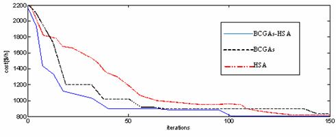
Figure 5. The function cost values in different iterations for BCGAs, HSA methods and BCGAs-HSA approach
Table 6 illustrates the results of the application of the methods BCGAs, HSA and BCGAs-HSA as well as the results of other researchers [17- 19] with the second case which is a study with constant losses.
Tables 5 and 7 illustrate the results of the application of the methods BCGAs, HSA and BCGAs-HSA with two other cases. The first study is a study ignoring losses; the second case is a study with variable losses (Third Variant).
These results clearly show the effectiveness and performance of the BCGAs-HSA over other methods either in terms of function cost value or in terms of convergence time as shown in Figure 5.
For the BCGAs only, convergence is reached after 145 iterations and the best cost is equal to 802.7719 $/hr, and for the HSA only the convergence is reached after 130 iterations and the best cost is equal to 802.4868 $/hr. Concerning the BCGAs-HSA hybrid technique the convergence is reached after 102 iterations and the cost reached is 801.3438 $/hr.
Conclusions
In this article we have applied a new approach that involves a combination of two Metaheuristic methods based on BCGAs and HSA.
We considered three cases; the first case without losses, the second by considering the constant losses, the third case with variable losses,
We have applied the approach to a network IEEE 30 nodes. The obtained results were compared to those of other researchers. The results show clearly the robustness and efficiency of the proposed approach in term of precision and convergence time.
References
1. Dommel H.W. Optimal power dispatch, IEEE Transactions on Power Apparatus and Systems, 1974, PAS93, p. 820-830.
2. Alsac O., Bright J., Prais M., Stott B., Further developments in LP-based optimal power flow, IEEE Transactions on Power Systems, 1990, 5, p. 697-711.
3. Nanda J., Kothari D.P., Srivatava S.C., New optimal power-dispatch algorithm using Fletcher’s quadratic programming method, In Proceedings of the IEE, 1989, 136, p. 153-161.
4. Younes M., Rahli M., Koridak H., Economic power dispatch using evolutionary algorithm, Journal of Electrical Engineering, 2006, 57(4), p. 211-217.
5.
6. Goldberg D.E., Genetic Algorithms in Search, Optimization and Machine Learning, Addison Wesley Publishing Company, 1989.
7. Younes M., Rahli M., Koridak L., Optimal Power Flow Based on Hybrid Genetic Algorithm, Journal of Information Science and Engineering, 2007, 23(3), p. 1801-1816.
8. Younes M., Hadjeri S., Sayah H., Dispatching économique par une méthode artificielle, Acta electrotehnica, 2009, 50(2), p. 128-136.
9. Radetic E., Pelikan M., Goldberg D.E., Effects of a deterministic hill climber on hBOA, Genetic and Evolutionary Computation Conference (GECCO-2009), pp. 437-444.
10. Michalewicz Z., A survey of constraint handling techniques in evolutionary computation methods, In Proceedings of the 4th Annual Conference on Evolutionary Programming, 1995, pp. 135-155.
11. Caorsi S., Massa A., Pastorino M., A computational technique based on a real-coded genetic algorithm for microwave imaging purposes, IEEE Trans. Geoscience and Remote Sensing , 2000, 38(4), p. 1697-1708.
12. Oyama A., Obayashi S., Nakamura T., Real-Coded Adaptive Range Genetic Algorithm Applied to Transonic Wing Optimization, Applied Soft Computing 2001, 1(3), p. 179-187.
13. Geem Z.W., Kim J.H., Loganthan G.V. A new heuristic optimization algorithm: harmony search, Simulation, 2001, 76(2), p. 60-68.
14. Yang X.S., Harmony Search as a Metaheuristic Algorithm in Music-Inspired Harmony Search Algorithm, Theory and applications SCI 191,2009, Zong Woo Geem (Ed.), 1-14,Springer-Verlag, ISBN 978-3-642-00184-0, Berlin Germany.
15. Fesanghary M., Mahdavi M., Minary M., Alizadeh Y., Hybridizing harmony search algorithm with sequential quadratic programming for engineering optimization problems, Comput. Methods Appl. Mech. Eng, 2008, 197(33-40), p. 3080-3091.
16. Yang X.-S., Harmony search as a metaheuristic algorithm, Music-inspired harmony search algorithm, 2009, p. 1-14.
17. Umapathy P., Venkataseshaiah C., Senthil Arumugam M., Particle Swarm Optimization with Various Inertia Weight Variants for Optimal Power Flow Solution, Discrete Dynamics in Nature and Society, 2010, Article ID 462145, 15 pp.
18. Alsac O., Stott B., Optimal load flow with steady-state security, IEEE Trans. Power Apparatus Syst., 1974, 93 (3), p.745-51.
19. Yuryevich J., Wong K.P., Evolutionary programming based optimal power flow algorithm, IEEE Trans Power Syst., 1999, 14(4), p. 1245-50.