High Order A-stable Continuous General Linear Methods for Solution of Systems of Initial Value Problems in ODEs
Dauda GuliburYAKUBU1*, Abubakar Muhammad KWAMI1, AbdulHamid Muhammad GAZALI2 and Abdu Ibrahim MAKSHA3
1Mathematical Sciences Programme, Abubakar Tafawa Balewa University, Bauchi, Nigeria.
2Department of Mathematics and Computer Science, FCE (Tech.) Gombe, Nigeria.
3Department of Mathematics and Computer Science, Federal Polytechnic, Mubi, Nigeria.
E-mails: daudagyakubu@gmail.com; Amkwamiatbu@yahoo.com; mohammedgazali01@yahoo.com & amaksha@yahoo.com
*Corresponding author: Phone: 2348052168433& 2348134168950
Abstract
Accurate solutions to initial value systems of ordinary differential equations may be approximated efficiently by Runge-Kutta methods or linear multistep methods. Each of these has limitations of one sort or another. In this paper we consider, as a middle ground, the derivation of continuous general linear methods for solution of stiff systems of initial value problems in ordinary differential equations. These methods are designed to combine the advantages of both Runge-Kutta and linear multistep methods. Particularly, methods possessing the property of A-stability are identified as promising methods within this large class of general linear methods. We show that the continuous general linear methods are self-starting and have more ability to solve the stiff systems of ordinary differential equations, than the discrete ones. The initial value systems of ordinary differential equations are solved, for instance, without looking for any other method to start the integration process. This desirable feature of the proposed approach leads to obtaining very high accuracy of the solution of the given problem. Illustrative examples are given to demonstrate the novelty and reliability of the methods.
Keywords
Block method; Continuous general linear method; Continuous scheme; Matrix inverse.
Introduction
In this paper we extend the idea of multistep collocation approach earlier used for the derivation of continuous general linear methods (CGLMs) [1-3], to derive high-order A-stable CGLMs for the numerical solution of stiff systems of initial value problems in ordinary differential equations (ODEs). Some concepts usually associated with the multistep collocation, like super-convergence (see, [4-6]) and now continuous schemes, have been endowed to the general linear methods. This can help to enlarge the scope of the CGLMs’ applications as it has been done with the finite difference methods and the finite element methods. General linear methods have played important role in many approximations of systems of ordinary differential equations, delay differential equations, as well as system of algebraic equations. In our approach to the multistep collocation, we have had an extensive experience and success with the following finite difference methods, namely, recursive formulation of Runge-Kutta methods (Gauss [7], Radau [8] and Lobatto [9]). These and many more will be considered in a future paper. Finally, we remark that our approach to multistep collocation has other desirable features. Firstly, it unifies many known and new classes of discrete linear multistep methods bringing the general linear methods which are probably the most simplest and convenient numerical methods for ODEs, under the banner of collocation derivation procedure. Secondly, for the existing systems of initial-value problems, automatic codes for the proposed continuous general linear methods (being continuous in nature) will be useful for step-size control, for variable-order and variable step codes.
Formulation of General Linear Methods
Traditionally methods for solving ordinary differential equations can be
categorize into two main classes: Runge-Kutta (multistage) methods and linear
multistep (multi-value) methods. Both of these classes have well known
advantages and disadvantages. In 1966, [10] first introduced general linear
methods as a unifying framework for the study of consistency, stability and
convergence of the traditional methods. Their formulations include both
multistage nature of Runge-Kutta methods as well as the multi-value nature of
linear multistep methods. General linear methods are characterized by four
matrices A, U, B, and V which make up a partitioned (s+r)×(s+r) matrix. Here,
for compactness of notations we write Y and F for the vector of Yi
and Fi values respectively, where ![]() is the approximation at the ith
internal stages and
is the approximation at the ith
internal stages and![]() . As with Runge-Kutta method, the vector
. As with Runge-Kutta method, the vector
![]() is
called the vector of abscissae. We also write y[n-1] for the
vector of approximations imported into step n and y[n] for
the quantities computed in this step and exported for use by the following
step. The detailed computation is based on the formula
is
called the vector of abscissae. We also write y[n-1] for the
vector of approximations imported into step n and y[n] for
the quantities computed in this step and exported for use by the following
step. The detailed computation is based on the formula
![]() (1)
(1)
for the stages and
![]() (2)
(2)
for the output
values, where I is the identity matrix of size equal to the differential
equation system to be solved. Also ![]() is the Kronecker product of two
matrices. With a slight notation, equations (1) and (2) are often written in
the form
is the Kronecker product of two
matrices. With a slight notation, equations (1) and (2) are often written in
the form
![]()
![]() M
=
M
= ![]() . (3a)
. (3a)
Hence it takes the form
 (3b)
(3b)
where s is the number of stages and r is the number of values passed from step to step. This formulation of general linear methods was first introduced by [11]. The structure of the leading coefficient matrix A, determines the implementation cost of these methods, similar to that of the matrix A in the Runge-Kutta methods. The V matrix determines the stability of these methods. The B matrix gives the weights. The U matrix is simply e.
In order for general linear methods to unify the study of the traditional
methods, (Runge-Kutta and linear multistep methods) it must be possible to
represent these traditional methods using the partitioned matrix M. As shown
in [12] Runge-Kutta methods are very simple to rewrite as general linear
methods. The matrix A of the general linear method is the same as the matrix A
of the Runge-Kutta method. The matrix B is bT where b is the vector
of weights of the Runge-Kutta method. Assuming the input vector is an
approximation to![]() , the U matrix is simply e, a vector of
ones in Runge-Kutta case. The V vector consists only of the number 1. It is
thus written as:
, the U matrix is simply e, a vector of
ones in Runge-Kutta case. The V vector consists only of the number 1. It is
thus written as:
![]()
![]() M =
M = 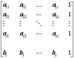 . (4)
. (4)
Runge-Kutta methods always have r =1, since only one quantity is passed from one step to the next. Similarly we can also easily represent the linear multistep methods in form of general linear methods.
For a linear k-step method [α, β] of the special form α(x) = 1-z, the natural way of writing this as a general linear method [12] is to choose r = k+1, s = 1 and the input approximations as

Definition 1.1. If a general linear method (A,U,B,V) takes the special form
![]()
![]()
where the rational function R(z) is known as the stability function of the method, then the method is said to have Runge-Kutta stability [13].
Definition1.2. A general linear method (A,U,B,V) is
A-stable if for all z![]() , I – zA is
non-singular and M(z) is a stability matrix [12].
, I – zA is
non-singular and M(z) is a stability matrix [12].
For methods with this property the step size is never restricted by stability on linear constant coefficient problems, regardless of the stiffness.
Definition1.3. A general linear method (A,U,B,V) is
L-stable if it is A-stable and ρ(M(![]() )) = 0 or the stronger condition M(
)) = 0 or the stronger condition M(![]() ) = 0 [13].
) = 0 [13].
Material and Method
Consider the general first order system of initial value problem of ordinary differential equations in the vector form
![]() (5)
(5)
where the solution y(x) satisfies additional initial or boundary conditions specified by (5) and whose generality is not a limitation to our formulation. A particularly useful class of discrete method for (5) is the class of linear multistep method of the form
![]() (6)
(6)
where k>0 is the step number, h is assumed (for simplicity of the analysis) to be a constant step-size given by h = xn+1– xn; hN = b - a; a = x0<…<xn<xn+1<…<xn+k<…<xN = b.
We consider an
approximant ![]() of the form in (6) formulated by [14]
which was a generalization of [5]
of the form in (6) formulated by [14]
which was a generalization of [5]
![]() (7)
(7)
defined over the
k-steps,![]() such that it satisfies the following
interpolation and collocation conditions
such that it satisfies the following
interpolation and collocation conditions
![]() j
j![]() {0,1,…,t-1} (8a)
{0,1,…,t-1} (8a)
![]() j
= 0,1,2,...,m-1 (8b)
j
= 0,1,2,...,m-1 (8b)
with ![]() and
and ![]() are assumed polynomials
in the form
are assumed polynomials
in the form
 j
j![]() {0,1,…,t-1} (9a)
{0,1,…,t-1} (9a)
![]() j
= 0,1,2,...,m-1 (9b)
j
= 0,1,2,...,m-1 (9b)
where t(t >
0) in (8a) are arbitrarily chosen interpolation points from ![]() and the collocation
points
and the collocation
points![]() in
(8b) are also taken from
in
(8b) are also taken from![]() .
.
From the interpolation and collocation conditions (8a)-(8b) and the
expression for![]() in (7), the following conditions are imposed
on
in (7), the following conditions are imposed
on ![]() (x),
and
(x),
and![]() (x):
(x):
 (10a)
(10a)
 . (10b)
Writing (10a)-(10b) in a matrix form, we have
![]() (11)
(11)
where I is an identity matrix of appropriate dimension,
 (12)
(12)
and
 (13)
(13)
are both of
dimension![]() .
It follows from (11) that the columns of C=D-1 give the continuous
coefficients
.
It follows from (11) that the columns of C=D-1 give the continuous
coefficients![]() (x), and
(x), and![]() (x). The matrix C is the
solution vector (output) and D is the non-singular matrix termed the Data
(input), which is assumed to be non-singular for the existence of the inverse
matrix C. An efficient algorithm for obtaining the elements of the inverse
matrix C is found in [14]. We now derive the continuous formulation of the
general linear methods following the derivation techniques discussed in section
3
(x). The matrix C is the
solution vector (output) and D is the non-singular matrix termed the Data
(input), which is assumed to be non-singular for the existence of the inverse
matrix C. An efficient algorithm for obtaining the elements of the inverse
matrix C is found in [14]. We now derive the continuous formulation of the
general linear methods following the derivation techniques discussed in section
3
Construction of the Continuous General Linear Methods
Here we propose a more computationally and attractive procedure, which leads to a class of A-stable continuous general linear methods for systems of stiff initial value problems. In this family, we consider the matrix D of the type in (12) see,[15] and equation (7), then using Taylor’s series method of expansion as done in the linear multistep methods we obtain our propose continuous scheme
![]() (14)
(14)
If we evaluate the proposed continuous scheme in (14), we first obtain the block finite difference method [15] associated with the continuous scheme and converted the block method into uniformly accurate order A-stable continuous general linear method and we display in the formalism of [16] as follows:
 (15)
(15)


 .
.
We plotted the region of absolute stability of the general linear method (15) using the method used in [17] and display in figure 1.
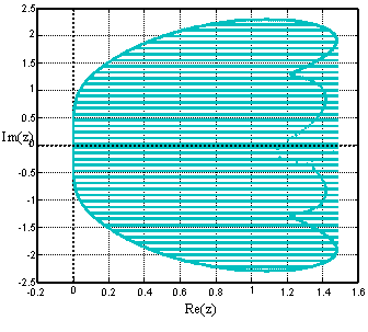
![]() Figure 1. Region of absolute stability of the CGLM (15) which
is A-stable and symmetric about x-axis
Figure 1. Region of absolute stability of the CGLM (15) which
is A-stable and symmetric about x-axis
Similarly for the high-order A-stable CGLM we obtain the propose continuous scheme
![]() (16)
(16)
from the inversion of the type of matrix D in (12), see [15], using computer algebra system, for example, Maple software package. Evaluating the proposed continuous scheme in (16) we obtain the uniformly accurate order block finite difference method, see [15] which was converted to CGLM.
 (17)
(17)


 .
.
We plotted the region of absolute stability of (17) following the method used in [17] and display the region as in figure 2
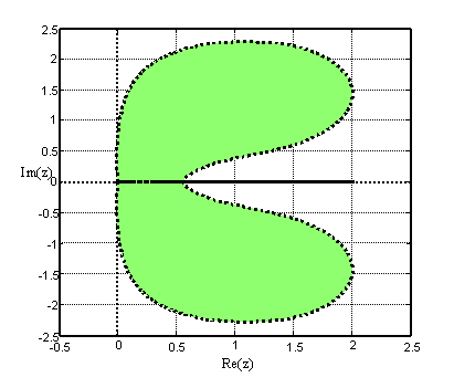
![]() Figure 2. Region of absolute stability of the CGLM (17) which
is A-stable and symmetric about x-axis
Figure 2. Region of absolute stability of the CGLM (17) which
is A-stable and symmetric about x-axis
Results and Discussion
In this section we present some numerical experiments to illustrate the performance of the newly constructed high-order A-stable CGLMs. All the computational programs were written in Matlab and implemented in the Mathematical Sciences Research and Development Laboratory, Abubakar Tafawa Balewa University, Bauchi, Nigeria. The test problems are some challenging systems of stiff initial value problems which have appeared in the literature. We compare the results obtained from the newly derived CGLMs with the results from some existing methods, for example, the Block Adams Moulton Method (BAMM) [15] and the GLM [1]. The absolute errors of the results obtained from the computed and exact solutions at some selected mesh points are shown in tables and the graphical plots are displayed in figures. The number of function evaluation (nfe) used in the computation is indicated in each problem.
Problem 1:
![]()
In the first problem we consider a real life problem of mathematical
models for predicting the population dynamics of competing species, one of which
is a predator, feeding on the other called a prey see [12]. If the numbers of
the species alive at time t are denoted by![]() and
and![]() , it is often assumed
that, the birth rate of each of the species is simply proportional to the
number of the species alive at that time and the death rate of each species
depends upon the population of both species. The population of the pair of
species is described by the equation in problem 1.We have solved the equation
and displayed the graphical plots in Figure 3.
, it is often assumed
that, the birth rate of each of the species is simply proportional to the
number of the species alive at that time and the death rate of each species
depends upon the population of both species. The population of the pair of
species is described by the equation in problem 1.We have solved the equation
and displayed the graphical plots in Figure 3.
Problem 2: Stiff nonlinear problem (The Kaps problem)
In the second problem, we consider the stiff nonlinear system of two dimensional Kaps problem taken from [12] with corresponding initial conditions
 .
.
The analytic solution is
 .
.
Solution of problem 1 using BAMM[15] , with nfe =100 Solution of problem 1 using GLM(15), with nfe =100
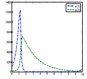
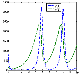
Solution of problem 1 using GLM [1] , with nfe =100 Solution of problem 1 using GLM(17), with nfe =100
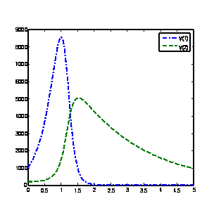
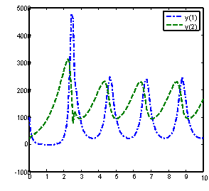
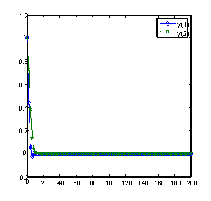
Figure 3. Computed solutions of problem 1 using BAMM [15] and the GLMs
The computed solutions of this problem using the newly derived CGLMs and some existing methods on the interval [0, 200] are displayed in figure 4. Even using a large number of functions evaluations per step the two newly derived methods perform very well compared to the other existing methods of the same order of convergence and of the same derivation.
Table 1. Absolute errors of numerical solutions of problem 2 within the interval 0 £ x £200
|
x |
BAMM[15] 1st Component y1 |
Method (15) 1st Component y1 |
GLM[1] 1st Component y1 |
Method(17) 1st Component y1 |
|
10.0 |
2.6156×10⁻⁴ |
4.5967×10⁻⁷ |
4.1584×10⁻⁶ |
7.4251 ×10⁻⁵ |
|
20.0 |
1.3911×10⁻⁸ |
7.7422×10⁻¹³ |
1.0689×10⁻¹³ |
4.6797×10⁻¹⁹ |
|
30.0 |
7.2173×10⁻¹³ |
2.9558×10⁻¹⁸ |
2.7477×10⁻²¹ |
2.0892×10⁻³² |
|
40.0 |
3.7435×10⁻¹⁷ |
9.4965×10⁻²⁴ |
7.0631×10⁻²⁹ |
9.3269×10-44 |
|
50.0 |
1.9417×10⁻²¹ |
3.0176×10⁻²⁹ |
1.8155×10-36 |
4.1638×10-57 |
|
60.0 |
1.0071×10⁻²⁵ |
9.5818×10⁻³⁵ |
4.6669×10-44 |
1.8589×10-70 |
|
70.0 |
5.2239×10⁻³⁰ |
3.0423×10-40 |
1.1996×10-51 |
8.2988×10-82 |
|
80.0 |
2.7095×10⁻³⁴ |
9.6594×10-46 |
3.0837×10-59 |
3.7049×10-95 |
|
90.0 |
1.4054×10-38 |
3.0669×10-51 |
7.9267×10-67 |
1.6540×10-108 |
|
100 |
7.2896×10-43 |
9.7376×10-57 |
2.0375×10-74 |
7.3840×10-120 |
Solution of problem 2 using BAMM [15] with nfe =100 Solution of problem 2 using method(15) with nfe =100
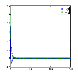
Solution of problem 2 using GLM [1] with nfe =100 Solution of problem 2 using method(17) with nfe =100
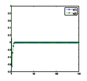
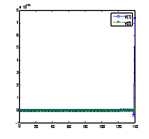
Figure 4. Computed solutions of problem 2 using BAMM [15] and the GLMs
Example 3: Stiff linear problem
The third example is another stiff system of three linear ordinary differential equations with corresponding initial conditions

where L = -25
and ![]() =
2.
=
2.
The analytic solution is
 .
.
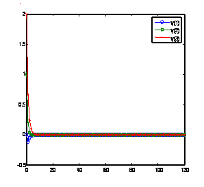
The results of using the newly constructed methods and some existing methods of the same order of convergence for the solution of this problem on the interval of [0,200] are presented in table 2 and the graphical plots are displayed in figure 6.
Table 2. Absolute errors of numerical solutions of problem 3 within the interval 0 £ x £200
|
x |
BAMM[15] 1st Component y1 |
Method (15) 1st Component y1 |
GLM[1] 1st Component y1 |
Method(17) 1st Component y1 |
|
10.0 |
2.7670×10⁻⁶ |
2.4086×10⁻⁵ |
1.4971×10⁻⁹ |
3.2272×10⁻¹² |
|
20.0 |
2.9527×10⁻¹² |
4.3083×10⁻¹¹ |
1.0331×10⁻¹⁸ |
1.0192×10⁻²⁷ |
|
30.0 |
8.1223×10⁻¹⁹ |
7.5150×10⁻¹⁷ |
8.4279×10⁻²⁶ |
3.2190×10-41 |
|
40.0 |
2.9775×10⁻²⁴ |
2.5262×10⁻²³ |
3.4871×10-36 |
1.0166×10-56 |
|
50.0 |
8.8571×10⁻³¹ |
6.6952×10⁻²⁹ |
4.9521×10-45 |
3.2109×10-70 |
|
60.0 |
2.0926×10-36 |
1.0165×10-36 |
2.7912×10-54 |
1.0140×10-85 |
|
70.0 |
2.0144×10-42 |
2.3383×10-41 |
3.9569×10-63 |
3.2027×10-99 |
|
80.0 |
1.0440×10-47 |
1.0188×10-48 |
1.2558×10-73 |
1.0115×10-114 |
|
90.0 |
6.8304×10-52 |
1.3595×10-54 |
1.6127×10-82 |
3.1946×10-128 |
|
100 |
4.8706×10-56 |
1.5936×10-59 |
6.8650×10-90 |
1.0089×10-143 |
Problem 4: The fourth problem is a stiff problem taken from [18].

The exact solution is: 
Solution of problem 3 using BAMM [15] with nfe =100 Solution of problem 3 using method(15) with nfe =100
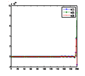
Solution of problem 3 using GLM [1] with nfe =100 Solution of problem 3 using method(17) with nfe =100
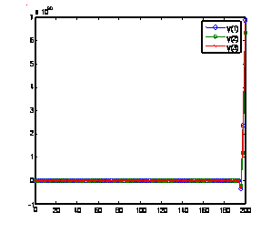
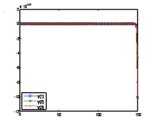
Figure 5. Computed solutions of problem 3 using BAMM [15] and the GLMs
Table 3. Absolute errors of numerical solutions of problem 4 within the interval 0 £ x £20
|
x |
BAMM [15] 1st Component y1 |
Method (15) 1st Component y1 |
GLM [1] 1st Component y1 |
Method (17) 1st Component y1 |
|
10.0 |
3.9452×10⁻⁴ |
1.9773×10⁻⁶ |
7.6043×10⁻¹⁰ |
4.2671×10⁻¹² |
|
20.0 |
6.5159×10⁻⁸ |
8.4968×10⁻¹² |
2.3050×10⁻²³ |
2.7547×10⁻²⁷ |
|
30.0 |
1.0761×10⁻¹¹ |
3.6510×10⁻¹⁹ |
6.9872×10⁻³⁵ |
1.7783×10-42 |
|
40.0 |
1.7772×10⁻¹⁵ |
1.5688×10⁻²⁶ |
2.1180×10-48 |
1.1480×10-57 |
|
50.0 |
2.9351×10⁻¹⁹ |
6.7414×10⁻³² |
6.4205×10-60 |
7.4114×10-71 |
|
60.0 |
4.8474×10⁻²³ |
2.8967×10-39 |
1.9462×10-73 |
4.7846×10-86 |
|
70.0 |
8.0055×10⁻²⁷ |
1.2447×10-46 |
5.8997×10-85 |
3.0887×10-101 |
|
80.0 |
1.3221×10⁻³⁰ |
5.3486×10-52 |
1.7883×10-98 |
1.9940×10-116 |
|
90.0 |
2.1835×10⁻³⁴ |
2.2983×10-59 |
5.4211×10-110 |
1.2872×10-131 |
|
100 |
3.6061×10-38 |
9.8758×10-65 |
1.6433×10-123 |
8.3102×10-145 |
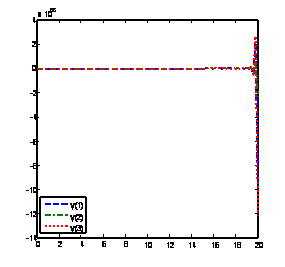
The eigenvalues of the system are λ1=-50 and λ2,3 = 0.1±8i. The eigenvalue λ2 give rise to sinusoidals with decaying amplitudes in the numerical solution, while the corresponding eigenvalue λ3 of the system give rise to sinusoidals with increasing amplitude. The solutions of the problem are presented in table 3 and the graphical plots are shown in figure 6.
Solution of problem 4 using BAMM [15] with nfe =100 Solution of problem 4 using method (15) with nfe =100
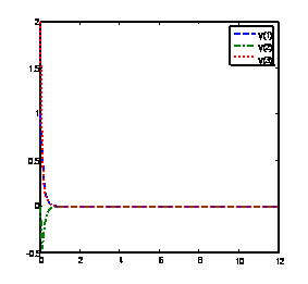
Solution of problem 4 using GLM [1] with nfe =100 Solution of problem 4 using method(17) with nfe =100
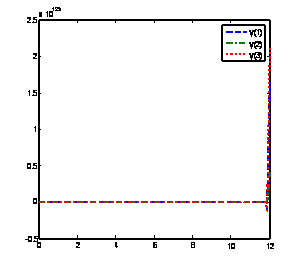
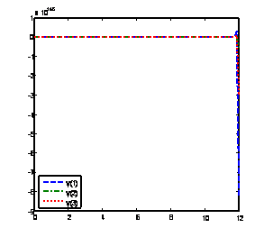
Figure 6. Computed solutions of problem 4 using BAMM [15] and the GLMs
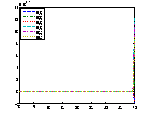
Problem 5: We consider another linear problem which is particularly referred to by [19] as a troublesome problem for some existing methods on which packages do exist, for example the DIFSUB of [20]. The eigenvalues of the Jacobian are λ1,2 = -10±100i, λ3 = -, λ4 = -1, λ5 = -0.5 and λ6 = -0.1. We consider solutions of the problem in the range 0 ≤ x ≤ 40.

The computed solutions are shown in table 4, while the graphical plots are displayed in figure 7.
Solution of problem 5 using BAMM [15] with nfe =100 Solution of problem 5 using method(15) with nfe =100
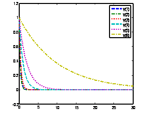
Solution of problem 5 using GLM [1] with nfe =100 Solution of problem 5 using method(17) with nfe =100
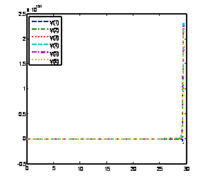
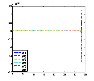
Figure 7. Computed solutions of problem 5 using BAMM [15] and the GLMs
The new approach considered in this paper is the use of more interpolation and collocation points in contracts to our previous papers [2,3] which extends some interpolations and collocations at the step points but with some evaluations at some selected off step points. In this way acceptable stability as for Runge-Kutta methods [12] is retained.
Table 4. Absolute errors of numerical solutions of problem 5 within the interval 0 £ x £40
|
x |
BAMM [15] 1st Component y1 |
Method (15) 1st Component y1 |
GLM [1] 1st Component y1 |
Method (17) 1st Component y1 |
|
10.0 |
1.8463×10⁻⁴ |
6.0231×10⁻¹⁰ |
7.3629×10⁻¹⁰ |
2.8465×10⁻¹² |
|
20.0 |
1.1360×10⁻⁸ |
3.1561×10⁻²² |
1.2813×10⁻²⁴ |
5.1603×10⁻²⁵ |
|
30.0 |
6.1893×10⁻¹³ |
1.6538×10⁻³⁴ |
2.2297×10-37 |
9.3548×10-38 |
|
40.0 |
2.9766×10⁻¹⁷ |
8.6663×10-45 |
3.8802×10-50 |
1.6958×10-52 |
|
50.0 |
1.2107×10⁻²¹ |
4.5412×10-57 |
6.7524×10-63 |
3.0744×10-65 |
|
60.0 |
3.5290×10⁻²⁶ |
2.3796×10-69 |
1.1750×10-77 |
5.5734×10-78 |
|
70.0 |
1.5124×10⁻³² |
1.2469×10-81 |
2.0448×10-90 |
1.0103×10-92 |
|
80.0 |
1.0889×10⁻³⁴ |
6.5341×10-92 |
3.5585×10-103 |
1.8316×10-105 |
|
90.0 |
1.1269×10-38 |
3.4239×10-104 |
6.1925×10-116 |
3.3205×10-118 |
|
100 |
8.3984×10-43 |
1.7941×10-116 |
1.0776×10-130 |
6.0196×10-131 |
Conclusion
All the derived methods obtained through this approach performed remarkably well in the solution of both stiff and non stiff systems of initial value problems (see, tables 1, 2 3, and 4). We plotted these solutions and compared them with the exact solutions or with solutions from other methods of the same order and same derivation, on the interval of consideration and there is remarkable agreement over very much longer intervals (see, figures 3, 4, 5, 6 and 7).
Reference
1. Yakubu D.G., Kwami A.M., Ahmed L.M., A special class of continuous General Linear Methods, J. of Computational and Applied Math., 2012, 31(2), p. 259-281.
2. Yakubu D.G., Gazali A.M., Dalatu P.I., Maksha A.I., A class of general linear methods with Runge-Kutta stability, J. Inst. Math. & Comput. Scie., 2009, 20, p. 9-20.
3. Yakubu D.G., Onumanyi P., Chollom J.P., A new family of general linear methods based on the block Adams-Moulton multistep methods, Journal of Pure and Applied Sciences, 2004, 7, p. 98-106.
4. Sirisena U.W., Onumanyi P., Yakubu D.G., Towards uniformly accurate continuous Finite Difference Approximation of ODEs, B. J. Pure and Appl Science, 2001, 1, p. 5-8.
5. Lie I., Nørsett S.P., Super-Convergence for multistep collocation, Math.Comp., 1989, 52, p. 65-80.
6. Zennaro M., One-step collocation; uniform super convergence; predictor-corrector methods. Local error estimates, SIAM. J. Numer. Anal., 1985, 22, p.1135-1152.
7. Yakubu D.G., Samaila M., Amina H., Kwami A.M., Symmetric Uniformly accurate Gauss Runge-Kutta Method, Leonardo Journal of Sciences, 2007, 11, p. 113-122.
8. Yakubu D.G., Hamza A., Tumba P., Kwami A.M., Uniformly accurate order five Radau-Runge-Kutta Collocation methods, Abacus Journal of the Mathematical Association of Nigeria, 2010, 37(2), p. 75-94.
9. Yakubu D.G., Manjak N. H., Buba S.S., Maksha A.I., A family of uniformly accurate order Lobatto-Runge-Kutta collocation methods, Journal of Computational and Applied Mathematics, 2011, 30(2), p. 315-330.
10. Butcher J.C. On the Convergence of Numerical Solution to Ordinary Differential Equations, Math. Comp. 1966, 20, p. 1 -10.
11. Burrage K., Butcher J.C., Non-linear stability for a general class of differential equation methods, BIT, 1980, 20, p. 185-203.
12. Butcher J.C., Numerical Methods for Ordinary Differential Equations, John Wiley and Son Ltd, 2003.
13. Butcher J.C., Numerical Methods for Ordinary Differential Equations, Second Edition, John Wiley and Son Ltd, 2008.
14. Onumanyi P., Awoyemi D.O., Jator S.N., Sirisena U.W., New linear Multi-step methods with continuous coefficients for first order initial value problems, Journal of the Nigerian Mathematical Society (JNMS), 1994, 13, p. 37-51.
15. Kwami A.M., A Special Class of Continuous General Linear Methods For Ordinary Differential Equations, Ph.D. Thesis, Abubakar Tafawa Balewa University, Bauchi, 2011, p. 47-60.
16. Butcher J.C., Wright W.M., Applications of doubly companion matrices, Applied Numer. Math., 2006, 56, p. 358-373.
17. Chollom J.P., Jackiewicz Z., Construction of two step Runge-Kutta (TSRK) methods with large regions of absolute stability, Compt. and Appl. Maths., 2003, 157, p. 125-137.
18. Lambert J.D., Numerical Methods for Ordinary Differential Systems, John Wiley, 1991.
19. Fatunla S.O., Numerical Integrators for Stiff and Highly Oscillatory Differential Equations, J. Mathematics of Computation, 1980, 34, p. 373-390.
20. Gear C.W., DIFSUB for solution of ordinary differential equations, Comm. ACM, 1971, 1, p. 185-190.