Applications of Cooperative Game Theory in Power System Allocation Problems

Fayçal ELATRECH KRATIMA^*, Fatima Zohra GHERBI, and Fatiha LAKDJA

Electrical Engineering Department. Intelligent Control and Electrical Power System Laboratory (ICEPS), Djillali Liabes University, Sidi-Bel-Abbes, 22000, Algeria.

E-mails: reseaukratima@live.fr; fzgherbi@gmail.com; flakdja@yahoo.fr

^* Corresponding author:^* Phone/Fax: 213 48 54 41 00

Abstract

This paper proposes a variant of cooperative game is derived and it has been proved that to determine the analytical solution to determine the nucleolus. The power generations or loads associated with the market are modeled as individual current injections based on a real-time solved AC power flow solution. Each load can be modeled as a current injection or equivalent constant impedance depending on whether it is required to be responsible for the system loss. Each current injection is then treated as an individual player of the transmission loss allocation game. The concept of Shapley value adopted from cooperative game theory is utilized to deal with the fairness of loss allocation. It has been applied to a 14-bus system and the results are discuses.

Keywords

Power system planning; Cooperative game theory; Shapley Value; Coalition formation; Transmission loss allocation.

Introduction

In the deregulated power market one of the most important issues is the allocation of transmission losses among market participants since system losses can typically represent significant portion of the total generation. The main difficulty of loss allocation is caused by the highly nonlinear and non-separable properties of the loss function. The electric power industry is undergoing a series of challenging changes due to deregulation and competition. One of the most important issues is the allocation of transmission losses among market participants since system losses can typically represent from five to ten percent of the total generation and costs millions of dollars per year. However, it is not a trivial task to “fairly” allocate a component of system losses to an individual participant of the market. The main difficulty of loss allocation is caused by the highly nonlinear and non-separable properties of the loss function. To deal with the loss allocation problem, a number of allocation schemes have been proposed in the literature. These schemes fall into the following categories: Prorate, proportional haring, incremental transmission loss, loss formula, and circuit theory. Some approaches are based on DC power flow, while some use AC load flow for matching the calculation results and actual power flows. Some schemes are branch-power-flow based, while some focus on the branch-current based allocation techniques.

Game theory provides well-behaved solution mechanisms with economic features for assessing the interaction of different participants in competitive markets and resolving the conflicts among players [1]. In particular, cooperative game theory is the most convenient tool to solve cost allocation problem [2, 3]. Some game theory based solutions have been proposed for power engineering problems, such as transmission cost allocation [1] and wheeling transactions [4]. The application of Shapley value concept arisen from the co-operative game theory was investigated to allocate losses and the work is extended in this paper. The transmission loss is derived as function individual current injections. Two basic formulations are presented to determine individual current injections. One basic model allocates losses only to the generators and the other allocates losses to both generators and loads. The main difference is that the former treats the load demands as equivalent constant admittances based on a real-time solved AC power flow solution and accordingly the bus admittance method impedance matrix (Ybus) is then modified, while the later formulates the load demands as equivalent current injections directly form bus impedance matrix.

Each current injection is then treated as an individual player of the transmission loss allocation game.

In the proposed approaches, the power generations and/or loads associated the market transactions are modeled as individual current injections [5]. Each current injection is then treated as an individual player of the transmission loss allocation game. The approaches are branch-current based, not branch-power-flow based. Without any approximations or assumptions like those made for a DC power flow or proportional sharing, the proposed approaches utilize the method of Shapley value [1] adopted from cooperative game theory to deal with the fairness issue of loss allocation. Some modified or alternative allocation approaches with or without a normalization procedure are also proposed to deal with the aggregated player of ancillary services and to speed up the computation when the number of players is large. The proposed approaches are consistent with the real-time AC power flow solution and recover the total system loss. The Kirchhoff’s laws and superposition principle are satisfied and both the network configuration and the voltage-current relationships are reflected. The interactions of players are naturally and fully considered. Moreover, the effect of reducing transmission loss can be identified from the negative loss allocation and the negative allocation can provide economic signals for the players.

Cooperative game will be described by the equations. These approaches (cooperative game) have been implemented and tested using the well-known IEEE14-bus system. A discussion about the significance, relevance, and usefulness of results obtained from these methods is presented,

Cooperative game

Consider an ‘n’ person balanced linear cooperative game described by the equations [6, 7]. The balanced game can be described as the solution vector satisfies all the collation constraints.

x(S) = ν(S)	(1)
x(N) = ν(N)	(2)

where x(S) is the set of possible coalitions and x(N) is the grand coalition.

Let the solution vector be

x = [x^·1, x^·2, ... x^·n-1, x^·n]

(3)

Then second order (quadratic) cooperative game which is described as follows.

minε(S)

Subject to

y(S) ≥ (ν(S))^2 + ε(S)	(4)
y(N) = (ν(N))^2	(5)

If the solution to the game is

y = [y^·1, y^·2, ... y^·n-1, y^·n]

(6)

Then the relation ship between the solution vectors is

y = ν(N)x

(7)

Multiply equations (1) by ν (N)

x(S)ν(N) = ν(S)ν(N)

(8)

In a balanced cooperative game it is understood that

x(S)Èx(S') = x(N)	(9)
ν(S) + ν(S') = ν(N)	(10)

where S' is the conjugate of coalition S

y(S) = (ν(S))^2 + ν(S)ν(S')	(11)
y(N) = (ν(N))^2	(12)

By comparing equations (4&11) the minimum value of the lexicographical excess vector is determined.

e(S) = ν(S) ν(S') = e(S')

(13)

Hence, it is proved and the proof can be extended to all coalition values which are real as well as complex numbers, which exhibits balancing condition. The equations 4&5 are modified for complex numbers

y(S) ≥ |ν(S)|^2 +ε(S)	(14)
y(N) = |ν(N)|^2	(15)

A. Generation and Load Models Based on a solved AC power flow solution for a pool based electric power market, let the complex power injection in to a generator bus i be  then the generation current injection is written as:

(16)

where V_i is its bus voltage. Similarly, let the complex power injection in to a load bus j be  we can then have load current injection

(17)

Or the equivalent load impedance

(18)

B. Transmission loss allocation problem

1. Loss allocation to generators only

For an ‘n’ node power network having ‘m’ generator buses the transmission loss of element ij connected between nodes ‘i’ and ‘j’ is derived in terms individual current contribution of each generator as

(19)

where  is the current contribution of ’k’^th generator to the element ‘ij’ and it can be determined from modified Y bus method using converged load flow solution.

is the resistance of line element ’ij’ connected between nodes ‘i’ and ‘j’. The individual voltage contribution of each generator is derived in terms of current injections.

(20)

is a square matrix of size ‘n’ and the columns m+1 to n will be zero since they are load buses.

2. Loss allocation to generators and loads

In this formulation loss allocation is made for generator as well as load buses. The individual voltage contribution of each bus is derived.

(21)

Now the transmission loss of ‘ij’th element in terms of individual current contribution is given:

(22)

For both methods the current contributions of ‘k’th bus for ‘ij’th element is

(23)

z_ij is the transmission line impedance of element ‘ij’ (pi model for transmission line is considered).

Since transmission loss is real the effect of shunt admittances can be ignored.

Now the current contribution of ‘k’th generator to element ‘ij’ is given by:

(24)

where z_ij is the transmission line impedance of element ‘ij’ (pi model for transmission line is considered). It can be observed that the branch current flowing through is the algebraic sum of individual current contributions of each generator

(25)

For each element ‘ij’ the coalitions present a balancing condition because of Kirchoff’s current law. Let ‘S’ be set of possible coalitions:

	(26)
	(27)

Let the solution vector for this balanced cooperative game be:

(28)

Now the coalition values for the transmission loss allocation problem is derived as:

	(29)
	(30)
	(31)
	(32)

The transmission loss contribution of ‘k’th generator to ‘ij’th element is determined as:

(33)

Now the transmission loss contribution of ‘k’th generator is the summation of losses to every line element of that generator.

(34)

The system parameters are shown in Tables 1, 2, 3

Table 1. Bus data of 14 bus system

Bus i	type	Pd	Qd	Gs	Bs	area	Vm	Va	baseKV	zone	Vmax	Vmin
1	3	0	0	0	0	1	1.06	0	0	1	1.06	0.94
2	2	21.7	12.7	0	0	1	1.045	-4.98	0	1	1.06	0.94
3	2	94.2	19	0	0	1	1.01	-12.72	0	1	1.06	0.94
4	1	47.8	-3.9	0	0	1	1.019	-10.33	0	1	1.06	0.94
5	1	7.6	1.6	0	0	1	1.02	-8.78	0	1	1.06	0.94
6	2	11.2	7.5	0	0	1	1.07	-14.22	0	1	1.06	0.94
7	1	0	0	0	0	1	1.062	-13.37	0	1	1.06	0.94
8	2	0	0	0	0	1	1.09	-13.36	0	1	1.06	0.94
9	1	29.5	16.6	0	19	1	1.056	-14.94	0	1	1.06	0.94
10	1	9	5.8	0	0	1	1.051	-15.1	0	1	1.06	0.94
11	1	3.5	1.8	0	0	1	1.057	-14.79	0	1	1.06	0.94
12	1	6.1	1.6	0	0	1	1.055	-15.07	0	1	1.06	0.94
13	1	13.5	5.8	0	0	1	1.05	-15.16	0	1	1.06	0.94
14	1	14.9	5	0	0	1	1.036	-16.04	0	1	1.06	0.94

Table 2. Generator data of 14 bus system

bus	Pg	Qg	Qmax	Qmin	Vg	mBase	status	Pmax	Pmin
1	232.4	-16.9	10	0	1.06	100	1	332.4	0
2	40	42.4	50	-40	1.045	100	1	140	0
3	0	23.4	40	0	1.01	100	1	100	0
6	0	12.2	24	-6	1.07	100	1	100	0
8	0	17.4	24	-6	1.09	100	1	100	0

Table 3. Branch data of 14 bus system

fbus	tbus	r	X	b	rateA	rateB	rateC	ratio	angle	status
1	2	0.01938	0.05917	0.0528	9900	1	1	1	0	1
1	5	0.05403	0.22304	0.0492	9900	1	1	1	0	1
2	3	0.04699	0.19797	0.0438	9900	1	1	1	0	1
2	4	0.05811	0.17632	0.034	9900	1	1	1	0	1
2	5	0.05695	0.17388	0.0346	9900	1	1	1	0	1
3	4	0.06701	0.17103	0.0128	9900	1	1	1	0	1
4	5	0.01335	0.04211	0	9900	0	1	1	1	1
4	7	0	0.20912	0	9900	0	0	0.978	0	1
4	9	0	0.55618	0	9900	0	0	0.969	0	1
5	6	0	0.25202	0	9900	0	0	0.932	0	1
6	11	0.09498	0.1989	0	9900	0	1	1	0	1
6	12	0.12291	0.25581	0	9900	0	1	1	0	1
6	13	0.03181	0.13027	0	9900	0	1	1	0	1
7	8	0	0.17615	0	9900	0	0	1	1	1
7	9	0	0.11001	0	9900	0	0	1	1	1
9	10	0.03181	0.0845	0	9900	0	1	1	0	1
9	14	0.12711	0.27038	0	9900	0	0	1	0	1
10	11	0.08205	0.19207	0	9900	0	0	1	0	1
12	13	0.22092	0.19988	0	9900	0	0	1	0	1
13	14	0.17093	0.34802	0	9900	0	0	1	0	1

Results and Discussions

Several systems have been used to test the proposed method. In this paper, the test results of a 14-bus system are presented and discussed.

The one-line diagram of a 14 bus system with 2 generation buses, 12 load buses, and 20 transmission lines is shown in Fig. 1. A solved power flow solution is shown in Table 1. The players of the loss allocation game are defined as the bus injected complex powers according to the solution listed in Table 4. The losses allocated to only generators and only loads for each transmission line and the total system loss allocations are listed in Tables 5 and 6, respectively.

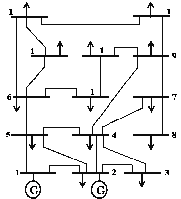
Figure 1. 14 bus system

The total allocated loss is consistent with the power flow solution and can reasonably reflect the amounts of transactions injected complex powers according to the solution listed in Table 7.

Since the network configuration and the location of each player are taken into account by the proposed schemes, the system loss is not evenly allocated to the supply side and the demand side. Thus, there is no need to specify the sharing factors of losses to be allocated to the supply side and demand side.

Table 4. Converged load flow solution of 14 bus system

Bus no	Voltage Mag pu	Voltage Angle Degrees	Real Power P(MW)	Reactive Power Q(MW)
1	1.0500	0	232.7115	-37.6883
2	1.0450	-5.2189	18.3000	51.0159
3	1.0100	-12.9697	-94.2000	6.7984
4	1.0165	-10.5354	-47.8000	3.9000
5	1.0175	-8.9813	-7.6000	-1.6000
6	1.0700	-14.4469	-11.2000	6.3182
7	1.0610	-13.5833	0.0000	0.0000
8	1.0900	-13.5833	0.0000	17.9653
9	1.0554	15.1618	-29.5000	-16.6000
10	1.0505	-15.3209	-9.0000	-5.8000
11	1.0567	-15.0151	-3.5000	-1.8000
12	1.0551	-15.3017	-6.1000	-1.6000
13	1.0503	-15.3817	-13.5000	-5.8000
14	1.0352	-16.2584	-14.9000	-5.0000
Transmission loss (MW)			13.71

Table 5. Transmission loss allocation (only generator buses)

Line N0:	G1 (MW)	G2 (MW)	Loss
1	4.5720	-0.0116	4.5604
2	2.7478	0.0481	2.7959
3	2.1419	0.1860	2.3279
4	1.5186	0.1596	1.6782
5	0.7953	0.1127	0.9080
6	0.3574	0.0189	0.3763
7	0.4964	0.0249	0.5213
8	0	0	0
9	0	0	0
10	0	0	0
11	0.0536	0.0029	0.0559
12	0.0674	0.0046	0.0720
13	0.1995	0.0135	0.2130
14	0	0	0
15	0	0	0
16	0.0114	0.0011	0.0125
17	0.1065	0.0086	0.1151
18	0.0126	0.0005	0.0126
19	0.0060	0.0004	0.0064
20	0.0520	0.0030	0.0550
Total	13.1384	0.5731	13.7115

Table 6. Transmission loss allocation (only load buses)

Line No	L3 (MW)	L4 (MW)	L5 (MW)	L6 (MW)	L7 (MW)	L8 (MW)	L9 (MW)	L10 (MW)	L11 (MW)	L12 (MW)	L13 (MW)	L14 (MW)
1	1.949	0.876	0.131	0.194	0.000	-0.010	0.550	0.168	0.065	0.111	0.249	0.279
2	0.890	0.595	0.112	0.162	0.000	0.000	0.392	0.120	0.048	0.086	0.188	0.205
3	1.678	0.236	0.027	0.042	0.000	-0.004	0.140	0.042	0.016	0.026	0.058	0.068
4	0.410	0.467	0.052	0.088	0.000	0.006	0.261	0.078	0.029	0.049	0.109	0.129
5	0.149	0.216	0.051	0.068	0.000	-0.003	0.157	0.049	0.020	0.037	0.080	0.084
6	0.677	-0.115	-0.012	-0.024	0.000	-0.009	-0.055	-0.016	-0.006	-0.011	-0.024	0.029
7	0.235	0.195	-0.016	-0.007	0.000	0.011	0.055	0.014	0.004	0.002	0.008	0.020
8	0.000	0.000	0.000	0.000	0.000	0.000	0.000	0.000	0.000	0.000	0.000	0.000
9	0.000	0.000	0.000	0.000	0.000	0.000	0.000	0.000	0.000	0.000	0.000	0.000
10	0.000	0.000	0.000	0.000	0.000	0.000	0.000	0.000	0.000	0.000	0.000	0.000
11	0.007	0.006	-0.001	-0.008	0.000	-0.008	0.042	0.021	0.015	-0.007	-0.015	0.004
12	0.001	0.001	0.000	-0.001	0.000	-0.002	0.007	0.001	0.000	0.032	0.021	0.012
13	0.006	0.005	-0.001	-0.007	0.000	-0.006	0.035	0.007	-0.001	0.017	0.101	0.057
14	0.000	0.000	0.000	0.000	0.000	0.000	0.000	0.000	0.000	0.000	0.000	0.000
15	0.000	0.000	0.000	0.000	0.000	0.000	0.000	0.000	0.000	0.000	0.000	0.000
16	-0.002	-0.001	0.000	0.001	0.000	0.003	-0.011	0.015	0.003	0.002	0.004	0.001
17	-0.008	-0.006	0.001	0.009	0.000	0.008	-0.045	-0.009	0.001	0.013	0.040	0.111
18	0.003	0.003	0.000	-0.004	0.000	-0.004	0.019	0.010	-0.006	-0.003	-0.007	0.002
19	0.000	0.000	0.000	0.000	0.000	-0.001	0.003	0.001	0.000	-0.009	0.008	0.005
20	0.006	0.005	-0.001	-0.008	0.000	-0.006	0.036	0.007	-0.001	-0.011	-0.032	0.058
Total	6.002	2.483	0.343	0.506	0.000	-0.025	1.585	0.508	0.186	0.333	0.787	1.005

Table 7. Transmission loss allocation (generator and load buses)

Line No	G1	G2	L3 (MW)	L4 (MW)	L5 (MW)	L6 (MW)	L7 (MW)	L8 (MW)	L9 (MW)	L10 (MW)	L11 (MW)	L12 (MW)	L13 (MW)	L14 (MW)
	(MW)	(MW)
1	4.139	-0.005	0.320	0.061	-0.002	0.002	0.000	0.007	0.017	0.005	0.002	0.002	0.005	0.008
2	2.290	0.049	-0.028	0.135	0.036	0.055	0.000	0.013	0.087	0.027	0.012	0.023	0.048	0.051
3	0.856	0.102	1.302	0.047	-0.004	-0.002	0.000	0.001	0.016	0.004	0.001	0.000	0.001	0.005
4	1.264	0.148	-0.145	0.188	0.006	0.021	0.000	0.009	0.081	0.023	0.008	0.012	0.027	0.038
5	0.572	0.104	-0.116	0.083	0.029	0.037	0.000	0.000	0.069	0.022	0.010	0.019	0.040	0.040
6	-0.200	-0.014	0.763	-0.071	-0.005	-0.012	0.000	-0.006	-0.031	-0.009	-0.003	-0.006	-0.013	-0.016
7	0.542	0.015	0.013	0.083	-0.034	-0.035	0.000	0.008	-0.011	-0.006	-0.004	-0.012	-0.023	-0.014
8	0.000	0.000	0.000	0.000	0.000	0.000	0.000	0.000	0.000	0.000	0.000	0.000	0.000	0.000
9	0.000	0.000	0.000	0.000	0.000	0.000	0.000	0.000	0.000	0.000	0.000	0.000	0.000	0.000
10	0.000	0.000	0.000	0.000	0.000	0.000	0.000	0.000	0.000	0.000	0.000	0.000	0.000	0.000
11	0.004	-0.002	0.006	0.005	-0.001	-0.008	0.000	-0.009	0.042	0.021	0.015	-0.007	-0.015	0.004
12	0.001	0.000	0.001	0.001	0.000	-0.001	0.000	-0.002	0.007	0.001	0.000	0.032	0.021	0.012
13	0.003	-0.001	0.005	0.005	-0.001	-0.008	0.000	-0.007	0.035	0.007	-0.001	0.017	0.101	0.057
14	0.000	0.000	0.000	0.000	0.000	0.000	0.000	0.000	0.000	0.000	0.000	0.000	0.000	0.000
15	0.000	0.000	0.000	0.000	0.000	0.000	0.000	0.000	0.000	0.000	0.000	0.000	0.000	0.000
16	-0.001	0.000	-0.001	-0.001	0.000	0.001	0.000	0.003	-0.011	0.015	0.003	0.002	0.004	-0.001
17	-0.004	0.002	-0.007	-0.006	0.001	0.009	0.000	0.009	-0.045	-0.009	0.001	0.013	0.040	0.111
18	0.002	-0.001	0.003	0.002	0.000	-0.004	0.000	-0.004	0.019	0.010	-0.006	-0.003	-0.007	0.002
19	0.000	0.000	0.000	0.000	0.000	0.000	0.000	-0.001	0.003	0.001	0.000	-0.009	0.008	0.004
20	0.003	-0.001	0.005	0.005	-0.001	-0.008	0.000	-0.006	0.036	0.007	-0.001	-0.011	-0.032	0.058
Total	9.471	0.396	2.120	0.535	0.025	0.048	0.000	0.015	0.314	0.118	0.035	0.072	0.206	0.357

Conclusions

The loss impacts between one player and any other coalitions of players are taken into account and the choice of cross term sharing factors is not uniform or arbitrary. Also, there is no need to specify the sharing factors of losses to be allocated to the supply side and demand side.

The branch with negative loss allocation may provide one interesting application on congestion management, which is currently under investigation

References

1. Gross G., Tao S., A physical-flow-based approach to allocating transmission losses in a transaction framework, IEEE Trans. PowerSyst, 2000, 15, p. 631-637.

2. Ding Q., Abur A., Transmission loss allocation in a multiple transaction framework, IEEE Trans. Power Syst, 2004, 19, p.214-220.

3. Leite da Silva A. M., Guilherme de Carvalho Costa J., Transmission loss allocation: part I – single energy market, IEEE Trans. Power Syst, 2003, 18, p. 1389-1394.

4. Zolezzi J. M., Rudnick H., Transmission cost allocation by cooperative games and coalition formation, IEEE Trans. Power Syst, 2002, 17, p. 1008-1015.

5. Hsieh S. C., Wang H. M., Allocation of transmission losses based on cooperative game theory and current injection models, in Proc.IEEE Int. Conf. Industrial Tech., Bangkok, Thailand, 2002, 11-14 ,p. 850-853.

6. Gross G., Tao S., A physical-flow-based approach to allocating transmission losses in a transaction framework, IEEE Trans. PowerSyst, 2000, 15, p. 631-637.

7. Saloman Danaraj, Shankarappa Kodad F., Tulsi Ram Das., Analytical solution to balanced quadratic cooperative game and its application to transmission loss allocation, Indian Journal of Science and Technology, 2007, Vol.1 No.2.

8. Krishna Deekshit  G., Poornachandra Rao N. , Transmission loss allocation in a multiple transaction framework, International Journal of Engineering Research and Applications (IJERA), May-Jun 2012, 2 (3), p.1944-1949.

9. Galiana F. D., Phelan M., Allocation of transmission losses to bilateral contracts in a competive environment, IEEE Trans. PowerSyst, 2000, 15, p. 143-150.

10. Conejo A. J., Arroyo J. M., Alguacil N., Guijarro A. L., Transmission loss allocation: a comparison of different practical algorithms, IEEE Trans. Power Syst, 2002, 17,  p. 571-576.

11. Gomez Exposito A., Riquelme Santos J. M., Gonzalez Garcia T., Ruiz Velasco E.A., Fair allocation of transmission power losses, IEEE Trans. Power Syst, 2000, 15, p. 184-188.

12. Daniel J. S., Salgado R. S., Irving M. R., Transmission loss allocation through a  modified Ybus,  IEE Proceedings- Generation, Transmission and Distribution, 2005, 152, p. 208-214.