Secured Economic Dispatch Algorithm using GSDF Matrix
Slimane SOUAG, Farid BENHAMIDA*
IRECOM Laboratory, Department of Electrical Engineering University of Djilali Liabes 22000, Sidi Bel Abbes, Algeria
E-mails: slimane.souag@gmail.com, farid.benhamida@yahoo.fr
* Corresponding author: Phone: +213666598556
Abstract
In this paper we present a new method for solving the secured power flow problem by the economic dispatch using DC power flow method and Generation Shift Distribution Factor (GSDF). A graphical interface in LabVIEW has been created as a virtual instrument. Hence the DC power flow reduces the power flow problem to a set of linear equations, which make the iterative calculation very fast and the GSFD matrix present the effects of single and multiple generator MW change on the transmission line. The effectiveness of the method developed is identified through its application to an IEEE-14 bus test system. The calculation results show excellent performance of the proposed method, in regard to computation time and quality of results.
Keywords
Economic Dispatch; Sensitivity Matrix; Power System; Virtual Instrument; Network Security; LabVIEW.
Introduction
The most accurate approach for modeling the steady state behaviour of balanced, three phase, electric power transmission networks is through the solution of the power flow [1]. With modern computers the power flow for even a fairly large system, such as the NERC 43,000 bus model of the North American Eastern Interconnect, can often be solved in seconds.
Solving this problem has led many researchers to find ways easier and faster to improve their convergence, reducing the execution time and save a lot of computer memory by using usually digital processes that can be classified into two groups:
(1) Iterative process: Gauss, Gauss Seidel, etc.
(2) Variationel process: Newton-Raphson method, or Jacobian.
However, the power flow solution can often be maddeningly difficult to obtain particularly when a good initial guess of the solution is not available. The flat start starting point taught to undergraduates for small systems not often works when solving realistic (large) systems. These convergence problems are especially troublesome when one tries to significantly change the operating point for a previously solved case, such as by scaling the load/generation levels.
The calculation of the power flow [2] is used to determine: (1) the complex tensions at different buses, (2) the transmitted power from one bus to another, (3) the powers injected in a bus and (4) real and reactive losses in the power system.
In this work, we were interested in monitoring the transmission line while working in economic dispatch mode; the power flow in the network can be estimated just using the DC (linearized) power flow method. But it is just a result; it is important to know what the value of the generator MW output is, and if a secured power flow in all the transmission line of the network can be make. It is also important to meet load demand at minimum operating total fuel cost, subject to equality constraints on power balance and inequality constraints on power outputs. This makes the ED problem a large-scale highly nonlinear constrained optimization problem. Improvements in scheduling of the generator power outputs can lead to very important fuel cost savings.
Material and Method
Economic dispatch
The basic economic dispatch can described mathematically as a minimization of problem [3].
|
|
(1) |
where Fi (Pi) is the fuel cost equation of the ith plant. It is the variation of fuel cost ($) with generated power (MW).
|
|
(2) |
If ai > 0 then the quadratic fuel cost function is monotonic. The total fuel cost is to be minimized subject to the following constraints.
|
|
(3) |
|
|
(4) |
|
|
(5) |
where, D is The real power load, Pi is the real power output at generator bus i, Bij, B0j, B00 are the B-coefficients of the transmission loss formula [4], Pimin is the minimal real power output at generator i, Pimax is the maximal real power output at generator i, PL is the transmission line losses, Fi is the fuel cost function of the generator i and N is the number of generators.
DC Power Flow Formulation
The simplification on fast decoupled Newton Raphson power flow algorithm [5] can be performed by neglecting simply any QV equation. This gives as result a linear and non-iterative power flow algorithm. To achieve these simplifications, we simply assume that |Vi| = 1 pu for every bus i.
And we have:
|
|
(6) |
The elements of matrices B are:
|
|
(7) |
|
|
(8) |
The terms of the matrix B are described above by Eq. (7) and Eq. (8). The dc power flow [6] is used only to calculate the real power flow (MW) of transmission lines and transformers. It gives no indication of the voltages or on the reactive power flow (Mvar) and apparent power (MVA).
The power flow on each line using the dc power flow can be described by the following equation:
|
|
(9) |
and
|
|
(10) |
Before moving on it is important to point out that one of the most obvious differences between the two the lack of losses in the DC solution can be reasonably compensated for by increasing the total DC load by the amount of the AC losses. Hence, in the DC approach the estimated transmission system losses could be allocated to the bus loads. This requirement to first estimate the losses is usually not burdensome since the specified total control area load is actually the true load plus the losses.
Generation Shift Distribution Factor (GSDF)
The affects of single and multiple generator MW change can be linearly approximately by calculating the state-independent GSDF [7]. Using the DC load flow model, the GSD Factor is expressed as:
|
|
(11) |
with m = 1, 2, , NL and NL is the number of lines.
where Pm is the real power flow on line m from sending bus j to receiving bus k; xm is the reactance of line m, is δj angle of bus j and Pgi is real power generated by the generator i.
From eq. (9) and (10), it is concluded that ∂δj/∂pgi = xji and ∂δk/∂pgi = xki thus,
|
|
(12) |
where xji and xki are the elements j-i and k-i of reactance matrix X of the lines, respectively where X = [0 x12 x13 x1n; x21 0 x23 x2n; ; xn1 xn2 0 ];
The GSDF matrix contains the GSDFs factor for all monitored lines [8], which represent a good sensitivity factor to generator MW change [9].
Solution Algorithm
To apply the secured economic dispatch, the line flows should be recomputed in each of the iteration due to the shifts in bus generation. In such kinds of applications, the total system demands are assumed remain unchanged but the losses are variable during iterations. If the loading levels change from the base point, a set of new line flow base should be established. In this process the GSDF matrix will be used to penalize the generator cost, the line that is overloaded they penalize the generators according to his sensitivity factor, this process will be repeated until the line problem is resolved [10].
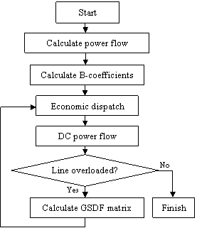
Figure 1. Secured economic dispatch algorithm flow chart
Algorithm Steps
Step 1: To start the algorithm all data of bus and lines must be known. It is also important to cheek if the total power demand is supported in the total addition of lines limits of the network.
Step 2: Calculate the power flow in the power system to get the flow in each line of the network and the output of the slack bus.
Step 3: Calculate the variable losses due to the change in generation output caused by the economic dispatch affectation.
Step 4: Execute the economic dispatch iteration to have the power allocation in each generation bus economically.
Step 5: Execution of the DC power flow must be performed to obtain the new power flow in the line due to the change in power output of generators.
Step 6: Check the lines limits [9], if there are no violations the algorithm will stop and the results are printed, if violations were observed the next step is executed.
Step 7: Calculate the generation shift distribution factor to have a sensitivity matrix of all lines flow to the change in each generators output.
Step 8: The GSDF matrix is used to penalize the cost of the generators who make the overload in the detected line and return to step 4 using the new generators cost, we repeat the loop up to have no overloaded line .
Step 9: If there are no overloaded line detected after step 5, the loop is stopped and the final results are printed.
Test System Data
The IEEE 14 bus system has different bus type coded as 1 for slack bus, 2 for PV bus and 0 for PQ bus (Table 1 & 2). The lines are coded by 0 and transformers by theirs tap changing. The cost data for this experiment are presented in Table 3.
Table 1. Bus data of IEEE 14 bus system
|
N° bus |
Type |
Voltage |
Angle |
Load MW |
Load Mvar |
Gen MW |
Gen Mvar |
Gen Qmin |
Gen Qmax |
Cond. |
Suscep. |
|
1 |
1 |
1.06 |
0 |
0 |
0 |
0 |
0 |
0 |
0 |
0 |
0 |
|
2 |
2 |
1.045 |
0 |
21.7 |
12.7 |
40 |
0 |
-40 |
50 |
0 |
0 |
|
3 |
2 |
1.01 |
0 |
94.2 |
19 |
0 |
0 |
0 |
40 |
0 |
0 |
|
4 |
0 |
1 |
0 |
47.8 |
-3.9 |
0 |
0 |
0 |
0 |
0 |
0 |
|
5 |
0 |
1 |
0 |
7.6 |
1.6 |
0 |
0 |
0 |
0 |
0 |
0 |
|
6 |
2 |
1.07 |
0 |
11.2 |
7.5 |
0 |
0 |
-6 |
24 |
0 |
0 |
|
7 |
0 |
1 |
0 |
0 |
0 |
0 |
0 |
0 |
0 |
0 |
0 |
|
8 |
2 |
1.09 |
0 |
0 |
0 |
0 |
0 |
-6 |
24 |
0 |
0 |
|
9 |
0 |
1 |
0 |
29.5 |
16.6 |
0 |
0 |
0 |
0 |
0 |
0.19 |
|
10 |
0 |
1 |
0 |
9 |
5.8 |
0 |
0 |
0 |
0 |
0 |
0 |
|
11 |
0 |
1 |
0 |
3.5 |
1.8 |
0 |
0 |
0 |
0 |
0 |
0 |
|
12 |
0 |
1 |
0 |
6.1 |
1.6 |
0 |
0 |
0 |
0 |
0 |
0 |
|
13 |
0 |
1 |
0 |
13.5 |
5.8 |
0 |
0 |
0 |
0 |
0 |
0 |
|
14 |
0 |
1 |
0 |
14.9 |
5 |
0 |
0 |
0 |
0 |
0 |
0 |
Table 2. Line data of IEEE 14 bus system
|
N° line |
From bus |
To bus |
R (pu) |
X (pu) |
1/2 B (pu) |
line code |
line Limits |
|
1 |
1 |
2 |
0.01938 |
0.05917 |
0.0264 |
0 |
200 |
|
2 |
1 |
5 |
0.05403 |
0.22304 |
0.0246 |
0 |
100 |
|
3 |
2 |
3 |
0.04699 |
0.19797 |
0.0219 |
0 |
100 |
|
4 |
2 |
4 |
0.05811 |
0.17632 |
0.017 |
0 |
100 |
|
5 |
2 |
5 |
0.05695 |
0.17388 |
0.0173 |
0 |
100 |
|
6 |
3 |
4 |
0.06701 |
0.17103 |
0.0064 |
0 |
50 |
|
7 |
4 |
5 |
0.01335 |
0.04211 |
0 |
0 |
100 |
|
8 |
4 |
7 |
0 |
0.20912 |
0 |
0.978 |
50 |
|
9 |
4 |
9 |
0 |
0.55618 |
0 |
0.969 |
50 |
|
10 |
5 |
6 |
0 |
0.25202 |
0 |
0.932 |
100 |
|
11 |
6 |
11 |
0.09498 |
0.1989 |
0 |
0 |
50 |
|
12 |
6 |
12 |
0.12291 |
0.25581 |
0 |
0 |
20 |
|
13 |
6 |
13 |
0.06615 |
0.13027 |
0 |
0 |
50 |
|
14 |
7 |
8 |
0 |
0.17615 |
0 |
1 |
50 |
|
15 |
7 |
9 |
0 |
0.11001 |
0 |
1 |
50 |
|
16 |
9 |
10 |
0.03181 |
0.0845 |
0 |
0 |
20 |
|
17 |
9 |
14 |
0.12711 |
0.27038 |
0 |
0 |
20 |
|
18 |
10 |
11 |
0.08205 |
0.19207 |
0 |
0 |
20 |
|
19 |
12 |
13 |
0.22092 |
0.19988 |
0 |
0 |
20 |
|
20 |
13 |
14 |
0.17093 |
0.34802 |
0 |
0 |
20 |
Table 3. Generator cost data of IEEE 14 bus system
|
Unit N° |
Pimin |
Pimax |
ai |
bi |
ci |
|
1 |
50 |
500 |
0.007 |
7 |
240 |
|
2 |
20 |
200 |
0.0095 |
10 |
200 |
|
3 |
20 |
300 |
0.009 |
8.5 |
220 |
|
4 |
20 |
150 |
0.009 |
11 |
200 |
|
5 |
20 |
200 |
0.008 |
10.5 |
220 |
The IEEE 14 Bus Test Case represents a portion of the American Electric Power System which is located in the Midwestern US as of February, 1962 [17]. Basically this 14 bus system has 14 buses, 5 generators and 11 loads presented in table 1 and 20 transmission lines and transformers presented in Table 2.
A better version is provided by Rich Christie at the
This section shows the most important case of the program, and the line power flow after the economic dispatch show the good state of all the lines (Figure 2-6), in this state the secured process is finished with zero security iteration it execute only the economic dispatch with total cost equal to 3415.99$/h shown in Figure 7.

Figure 2. Bus and line data of IEEE 14 bus system in LabVIEW program
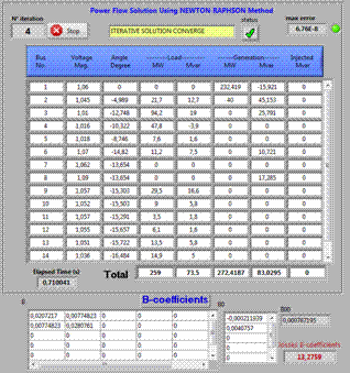
Figure 3. Power flow of IEEE 14 bus system in LabVIEW program

Figure 4. Cost data of IEEE 14 bus system in LabVIEW program
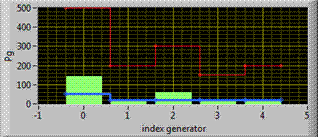
Figure 5. Economic dispatch of IEEE 14 bus system in LabVIEW
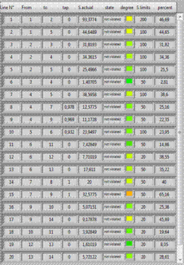
Figure 6. Line power flow of IEEE 14 bus system in LabVIEW program
To show the efficiency of the secured economic dispatch to resolve the problem of line overloaded, we increase the total MW load in the system to cause en overload in one or multiple lines, by make some adjustments in bus 4 and 5, and add to each bus 100 MW of load and see what it gives (Figure 7).

Figure 7. Economic dispatch results of IEEE 14 generation system in LabVIEW
Results and Discussion
In this section the same IEEE 14 bus system is texted by adjusting the load of bus 4 and 5, the total MW load will be increase to 459 MW to cause an overload in lines and resolve it by the new algorithm.
We have implemented our algorithms in the LABVIEW power system simulation package LABPOWER and verified them on the IEEE power system test cases [17] with the modified load demands. All experiments are conducted on a Windows 7 with 2.66 GHz DUO CPU and 4G RAM.
The new adjustment of the load caused a multiple overload in the network shown in figure 8; before test the new algorithm we will make a simple economic dispatch in the network to save some money and look what will happen in the line flow state [11], certainly there will be a new power distribution.
The new values of powers generated make in figure 9 the new state of the lines power flow after the execution of the economic dispatch, look that the problem is slightly improved but we have always an overload in the line number 6; some problem is solved, but it is by chance.
To solve the problem we must face set and include a verification process and measured the sensitivity with respect to different party involved, and this is what our new algorithm is doing.
There are many theories for finding the best compromise solutions between the economic dispatch and secured power flow, and most of this solution includes the security as constraint in the process of economic dispatch which will transform to a strongly constrained nonlinear optimization, particularly when there are a large number of transmission lines. Hence the solution is not always guaranteed, or it will be found after many iterations.
Finally we execute the new algorithm to resolve problem in the network economically using the GSDF matrix which will be calculated just after the economic dispatch [12].
Innovation in this algorithm is to preserve the economic dispatch as it is (Figure 8), and added a process that will economically penalize generator according to their impact on safety on the grid. ie the generator causing more overload on the line reported it will be considered more expensive and automatically the process of the economic dispatch will reduce the production of the latter.
The GSDF value correspond to each line power flow sensitivity to each generator power output [13], will penalize the cost of the latter will he have forced to produce less and therefore decrease the power in overloaded line [14].
Figure 9 showed that after the execution of the new algorithm in the overloaded system [15], the total cost of production is slightly increased and this is normal because it is a system constraints but the problem is directly resolved after 2 security iteration which proves the efficiency and speed of this algorithm (Figure 10 and 11). This algorithm was tested on more complex and large system and it showed a very large facility resolution [16].
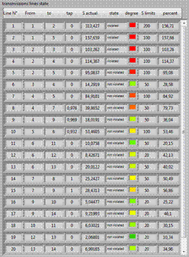
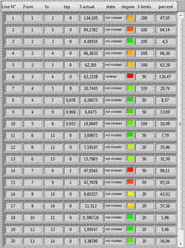
Figure 8. Line power flow of the adjusted IEEE 14 bus system before (left) and after (right) economic dispatch
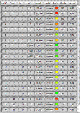
Figure 9. Line power flow of the adjusted IEEE 14 bus system after the secured economic dispatch

Figure 10. Economic dispatch results of adjusted IEEE 14 bus system with just economic dispatch in LabVIEW

Figure 11. Economic dispatch results of adjusted IEEE 14 bus system with secured economic dispatch in LabVIEW
In this paper, we have proposed a novel algorithm to solve economic and security problem in the network. We have also integrated the sensitivity matrix with the contingency constrained economic dispatch problem. With such extension, the original economic dispatch problem becomes a difficult optimization problem. We then propose an elegant way to transform the problem as a more tractable problem by adopting the GSDF matrix element as penalty factor of the generators who make overload in reported lines. They preserve the network in a good state of power flow and preserve a good price of generation cost.
The results showed using this algorithm are satisfactory, which checks the validity of this study concerning the execution time. The performance of our method is much faster.
In the future, we will further study how to take the variation of load into consideration, the value of which also varies with time and locations.
Conclusion
Our experiments based on IEEE power system test cases have shown that the proposed algorithm can achieve speed-up at a similar generation cost when compared to the conventional practice.
References
1. Overbye T. J., Cheng X., Sun Y., A
Comparison of the AC and DC Power Flow Models for LMP Calculation,
Published in the Proceedings of the Hawaii International Conference on System
Sciences, Big Island.
2. Souag S., Calcul des B-coefficients sous LabVIEW, M.Sc. Thesis, University Djillali Liabessidi bel Abbes, Jun 2011.
3. Kothari D. P., Dhillon J. S, Power System Optimization, PHI Learning Pvt. Ltd. 2004.
4. Kothari D. P., Nagrath I. J.T., Modern power system analysis, McGraw-Hill Education, 2003.
5. Wood A. J., Wollenberg B. F., Power
Generation Operation and Control. 2nd Edition, John Wiley & Sons,
6. Souag S., Benhamida F. A., Virtual Instrument for Dc Power Flow Solution Using Labview Language, Advances in Electrical and Electronic Engineering, 2012, 10(02), p. 68-74.
7. Sauer P. W., On the formulation of power distribution factors for linear load flow methods, IEEE Trans. on Power Apparatus and Systems, 1981, 100(2), p. 764-770.
8. Scott R., Dahman P. E., Power World Corporation. N-1-1 Contingency Analysis using PowerWorld Simulator, PowerWorld Client Conf., Jun. 2010, Portland, Oregon.
9. Mishra V. J., Khardenvis M. D., Contingency analysis of power system, in Proc. 2012 IEEE Students' Conf. on Electrical. Electronics and Computer Science (SCEECS), 2012, p. 1-4.
10. Henneaux P., Labeau P. E., Maun J. C., Blackout Probabilistic Risk Assessment and Thermal Effects: Impacts of Changes in Generation, IEEE transactions on power systems. 2013, 28(4), p. 4722-4731.
11. Romero N. R., Nozick L. K., Dobson I. D., Xu N., Transmission and Generation Expansion to Mitigate Seismic Risk, IEEE Transactions on Power Systems, 2013, 28(4), p. 3692-3701.
12. Verma K., Niazi K. R., Contingency Constrained Power System Security Assessment using Cascade Neural Network, Journal of Electrical Systems, 2012, 8(1), p. 1-12.
13. Su C.-L., Distribution Probabilistic Load Flow Solution Considering Network Reconfiguration and Voltage Control Devices, 15th PSCC. Liege, 2005, p. 22-26.
14. Rudnick H., Mocarquer S., Andrade E., Vuchetich E., Miquel P., Disaster management restoring electricity supply after the 2010 Chilean earthquake, IEEE Power and Energy Magazine, 2011, 9(2), p. 37-45.
15. Brown N. J. K., Gearhart J. L., Jones D. A., Nozick L. K., Xu N., Romero N., Optimizing the selection of scenarios for loss estimation in transportation networks, In Proc., 2011, Winter Simulation Conf: Simulation for a Sustainable World.
16. Henneaux P., Labeau P.-E., Maun J.-C., A level-1 probabilistic risk assessment to blackout hazard in transmission power systems, Reliability Engineering & System Safety, 2012, 102, p. 41-52.
17. Power Systems Test Case Archive [online], Available at: http://www.ee.washington.edu/research/pstca/pf14/pg_tca14bus.htm


