Optimal sensors placement for monitoring a steam condenser of the distillation column using bond graph approach
Samia LATRECHE*, Mohammed MOSTEFAI, Mabrouk KHEMLICHE
Automatic Laboratory of Setif, Electrical Engineering Department, University of Setif 1, 19000, Setif, Algeria
E-mails: ksamia2002@yahoo.fr, mostefai@univ-setif.dz, mabroukkhemliche@yahoo.fr
* Corresponding author, Phone: +213668769714; Fax: +213 36 92 51 02
Abstract
This paper deals with monitoring of a process engineering system. The steam condenser was monitored by bond graph tool. The model was constituted by nine capacitive and resistive elements which needed minimum of sensors. This method was based on Analytical Redundancy Relations which were generated from a condenser model and represented residuals. After substitution, we obtained the placement of six sensors which guaranteed the monitoring of nine components. A fault is created by the abrupt annulment of the fluid flow value provided by the source. The block diagram is elaborated on SYMBOLS software and we supervised the residuals evolution.
Keywords
Optimization; Sensors placement; Monitoring; Condenser; Distillation Column; Bond graph
Introduction
The monitoring system with rigid structure knows progress during the last years. The monitoring of the thermal system is difficult because of the phenomenon complexity [1]. These industrial processes have a strongly nonlinear behaviour due mainly to the mutual interaction of several phenomena with various nature and the association of the technological components. The system modelled and monitored, is a condenser of the distillation column which is produced thermal, chemical and hydraulic phenomena. In this case, the bond graph tool reduces all difficulties because of its causal and structural properties. After the validation of the model, the placement of the sensors, is made and followed by the research of the optimal case [2], and [3]. The advantages of applying bond graph model to the condenser of distillation column are the ability to build a graphical circuit, the use of detailed equations, the encapsulation of pieces of the model into sub-models and the representation of the system power flows in details. The main drawback of using bond graphs is that they cannot describe distillation equations. In this work, both bond graph modelling and monitoring by sensors placement are proposed for a condenser of a distillation column.
Description of the system
The condenser schematic is shown in Figure 1. The steam enters at the left side, condensed on the pipes filled with cooling water.
It falls to the floors and leaves from there to the receiver through control valves [1]. The water outflow (condensate) is controlled by three valves in order to keep its level constant. The condenser is a module of four input-outputs. It is composed by a coolant circuit made up of a unit of pipes which lead the liquid. The liquid phase of cold fluid accumulates heat while passing in steam (vapor) phase. When the steam flow attempts the condenser, a contact is obtained between the steam and the pipes of the fluid circuit in which circulate both the cold fluid and the steam condensed in fine droplets which are formed at the condenser bottom [4].
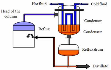
Figure 1. The condenser operating in the distillation column
Steam circulating in the column is from a portion of the feed when it is vaporized. In the boiler, the liquid mixture of the beginning is heated for the vaporizer. The steam which arrives in the line of column heading is condensed completely or partially by a condenser [5], [6]. When the steam arrives in contact with the fluid pipes in which circulates a cold fluid, it was condensed in liquid which runs out downwards by simple gravity and collected at the bottom of the condenser. The liquid obtained is generally returned in the column under the name of backward flow by tubular of feed. The other part is collected like a distillate and the non-vaporized part comes to contribute to the liquid flow. The operation is repeated, by ensuring the condensation of the steam of column heading [2].
Sensors placement algorithm
This procedure consists of an optimal sensors placement for the components monitoring, i.e. to detect and to isolate the components failures. From a physical process we elaborate a bond graph model. In bond graph model, sensors are placed only at the junction 0 and 1, we consider a virtual placement of the sensor at the position j, which is represented by the variables x and y. N0, and N1 are respectively the junction numbers 0Ci, 1Rj. i, j, n and m are respectively the junction orders, the number of the bonds’ fixed on the junction 0Ci, 1Rj. The structural equations of the junction s0Ci, which describe the effort equality and the pressure conservation produced in C element, are given by (1).
|
|
(1) |

where fk and ek
are respectively the flow and the effort of the junction number k; ak=+1
if the bond graph semi flow is toward junction; ak=-1
otherwise. For the nonlinear functions ФCi and s the
|
|
(2) |

where i=1, N0 ; Dei effort detectors, xi binary variables xi=1 if we place detector; xi=0 otherwise. The structural equations of the junctions 1Rj are given by equation (3).
|
|
(3) |

For the nonlinear functions ФRj, the flow and effort variables are determined by (4):
|
|
(4) |

where j=1, N1; Dfj flow detectors, yj binary variables yj =1 if we place detector; yj =0 otherwise. The combinations of the variables xi and yj make it possible to generate analytical redundancy relations which give the structures of the residuals. The bond graph model of the condenser in the distillation column representing hydraulic and thermal phenomena with steam and liquid phases and using sensors placement (effort and flow detectors) is represented by Figure 2. This model is composed by 5 junctions type 0 attached to 5 components CV, CL, CT1, CT3 and CTS noted 01, 02, 03, 04, 05 and 4 junctions type 1 attached to 4 components RT1, RT3, RTS and R noted 11, 12, 13, 14 [2]. These components are: CV the pipe capacity traveled by fluid in vapor phase, CL the pipe capacity of fluid in liquid phase; CT1 the tank1 capacity; CT3 the tank3 capacity; CTS the tank capacity of a distillate; RT1, RT3, RTS and R are respectively, the valves of tank1 and tank3, the distillate and the reflux drum.
Table 1. Nomenclature
|
Variables |
Bond graph descriptions |
Physical descriptions |
|
E |
Effort |
Pressure P, Temperature T |
|
F |
Flow |
Masse flow dm/dt, Enthalpy flow dH/dt |
|
De |
Effort detector |
Measured effort |
|
Df |
Flow detector |
Measured flow |
|
Se, MSe |
Effort source |
Thermal or Hydraulic effort |
|
Sf, MSf |
Flow source |
Thermal or Hydraulic flow |
|
R |
Resistive component |
Valve |
|
C |
Capacitive component |
Tank |
|
ARR |
Analytical Redundancy Relation |
Residual (Failure indicators) |
|
S |
Derivative operator |
d/dt |
|
1/s |
Integral operator |
∫dt |
|
Φ |
Nonlinear components evolution |
ΦR; ΦCV; ΦCL; ΦCT1; ΦCT3; ΦCTS; ΦRT1; ΦRT3; ΦRTS |
|
CV |
Vapour (steam) capacity |
Pipe capacity travelled by fluid in vapour phase |
|
CL |
Liquid capacity |
Pipe capacity travelled by fluid in liquid phase |
|
CT1 |
Tank1 capacity |
Level of fluid into tank1 |
|
CT3 |
Tank3 capacity |
Level of fluid into tank3 |
|
CTS |
Capacity of distillate tank |
Distillate into reflux drum |
|
RT1 |
Tank1 resistor |
Valve of fluid into tank1 |
|
RT3 |
Tank3 resistor |
Valve of fluid into tank3 |
|
RTS |
Resistor of distillate tank |
Distillate valve |
The bond graph model is described as follows:
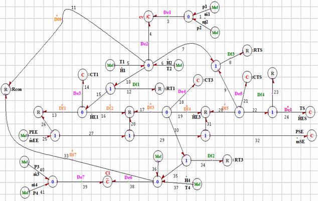
Figure 2. Bond graph model of the condenser with sensors placement
Constitutive and structural equations
The calculation of the residuals needs application of the previous algorithm by generating flow f and effort e of all junctions. For example, the junctions 0De1 and 1Df1 are described by the equations (5) and (6).
|
|
(5) |
|
|
(6) |


where Msf1 and Msf2 represent the controlled (modulated by signals) flow source of bond 1 and bond 2. From the previous equations we can deduce the system (7) which permits us to generate residuals:
|
|
(7) |
Optimization technique
The equations above allow according to binary variables xi and yj determining the final system structure to supervise. The optimal case is with how many sensors to supervise this model. There exist 2n = 29 = 512 combinations to obtain the optimal case.
From the combination with 9 sensors placed in the 9 positions, the ARRs are calculated until to obtain the optimal combination. The detection is defined by columns of the signature table different to zero. The isolation is guaranteed by the columns different each other.
In the second step, the substitution is used to reduce the number of ARRs and to verify the monitoring from the signature table. In our case, 6 ARRs satisfied that all the components are monitored. The generated ARRs are given by the following relations (the sensors are placed only if xi and yj = 1).
Substitution with 9 sensors
All the sensors are placed, so each component is monitored by one sensor and the system (7) becomes as follows for [x1 y1 x2 y2 x3 y3 x4 y4 x5 x6 x7]T = [11011111110]T
|
|
(8) |
Table 2. Faults signature table for 9 detectors
|
|
CV |
CL |
CT1 |
RT1 |
CT3 |
RT3 |
CTS |
RTS |
R |
|
ARR1 |
1 |
|
|
|
|
|
|
|
|
|
ARR2 |
1 |
|
|
1 |
|
|
|
|
|
|
ARR3 |
|
|
|
|
|
1 |
|
|
|
|
ARR4 |
|
|
1 |
|
|
|
|
|
|
|
ARR5 |
1 |
|
|
|
|
|
|
1 |
|
|
ARR6 |
|
|
|
|
1 |
|
|
|
|
|
ARR7 |
|
|
|
|
|
|
|
|
1 |
|
ARR8 |
|
|
|
|
|
|
1 |
|
|
|
ARR9 |
1 |
|
|
|
|
|
|
|
|
In this case faults on all the components are detectable and localizable.
Substitution with 8 sensors
One of the possible combinations is chosen, so 8 ARRs are generated for monitoring 9 components. The combination used in the system (7) is [01101111110]T.
|
|
(9) |
Table 3. Faults signature table for 8 detectors
|
|
CV |
CL |
CT1 |
RT1 |
CT3 |
RT3 |
CTS |
RTS |
R |
|
ARR1 |
|
|
|
1 |
|
|
|
|
|
|
ARR2 |
1 |
|
|
|
|
|
|
|
|
|
ARR3 |
|
|
1 |
|
|
|
|
|
|
|
ARR4 |
|
|
|
|
|
|
|
1 |
|
|
ARR5 |
|
|
|
|
1 |
1 |
|
|
|
|
ARR6 |
|
|
|
|
|
|
|
|
1 |
|
ARR7 |
|
|
|
|
|
|
1 |
|
|
|
ARR8 |
|
1 |
|
|
|
1 |
|
|
|
In this case faults on all the components are detectable and isolable.
Substitution with 7 sensors
Not localizable case [01000111111]T
|
|
(10) |
Table 4. Faults signature table for 7 detectors
|
|
CV |
CL |
CT1 |
RT1 |
CT3 |
RT3 |
CTS |
RTS |
R |
|
ARR1 |
1 |
|
1 |
1 |
|
|
|
|
|
|
ARR2 |
|
|
|
|
1 |
1 |
|
|
|
|
ARR3 |
|
|
|
|
|
|
|
|
1 |
|
ARR4 |
|
|
|
|
|
|
1 |
|
|
|
ARR5 |
|
|
|
|
|
|
1 |
|
|
|
ARR6 |
|
1 |
|
|
|
|
|
|
|
|
ARR7 |
1 |
|
|
|
|
|
|
1 |
|
The fault on (CT1 and RT1) and the fault on (CT3 and RT3) are not localizable (the same column vectors).
Detectable and isolable case [00101111110]T
|
|
(11) |
Table 5. Faults signature table for 7 detectors
|
|
CV |
CL |
CT1 |
RT1 |
CT3 |
RT3 |
CTS |
RTS |
R |
|
ARR1 |
1 |
|
|
1 |
|
|
|
|
|
|
ARR2 |
|
|
1 |
|
|
|
|
|
|
|
ARR3 |
|
|
|
|
|
|
|
1 |
|
|
ARR4 |
|
|
|
|
1 |
1 |
|
|
|
|
ARR5 |
|
|
|
|
|
|
|
|
1 |
|
ARR6 |
|
|
|
|
|
|
1 |
|
|
|
ARR7 |
|
1 |
|
|
|
1 |
|
|
|
Substitution with 6 sensors [01001111010]T
|
|
(12) |
Table 6. Faults signature table for 6 detectors
|
|
CV |
CL |
CT1 |
RT1 |
CT3 |
RT3 |
CTS |
RTS |
R |
|
ARR1 |
1 |
|
|
1 |
|
|
|
|
|
|
ARR2 |
|
|
1 |
|
|
|
|
|
|
|
ARR3 |
1 |
|
|
|
|
|
1 |
1 |
|
|
ARR4 |
|
|
|
|
1 |
1 |
|
|
|
|
ARR5 |
|
|
|
|
|
|
1 |
|
1 |
|
ARR6 |
|
1 |
|
|
|
1 |
|
|
|
All the combinations with 5 sensors placed cannot ensure the detection and the isolation of the failures that affect this system. The optimal case is to monitor 9 components by only 6 sensors.
The table (6) of the residuals structure permit to notice that the residuals structures are different and the faults signatures are different and not equal to zero, thus the components CV, CL, CT1, RT1, CT3, RT3, CTS, RTS and R are monitored.
Sensitivity of the detectors
Under normal operating, the residuals must be constantly equal to zero but it is not always the case because of the modelling errors and the unavailability of the technical specifications of the real system.
From SYMBOLS software (System Modelling Bond graph Language Simulation), we have implanted the bond graph model [5] associated to the block diagram of the ARR that contain affected components.
We create fault on RT1 component monitored by the detector Df1 (disturbance from the association of Dirac pulse and Unit echelon). Their values are not considered only their appearances in the relation are taking into account with evaluation term (1 for the presence and 0 for the absence).
In the first time, the fault is created between the instant t1=2s and t2=2.01s by the annulment of fluid flow provided by the source [9], [10].
In the second time, the block diagram of the ARR1, ARR2 and ARR3 expressions that contain Df1 detector (see Figure. 3) is elaborated. The three outputs are represented by three scopes.
The failure is injected on 1RT1 junction monitored by the detector Df1 (Figure. 4) and not sensitive to ARR4, ARR5 and ARR6 (Figure. 5). It represents sealing in the valve and leakage in the tank.
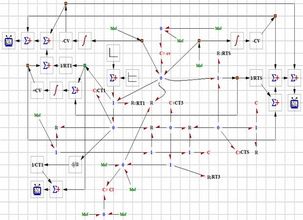
Figure 3. Block diagram representing the ARRs function of Df1
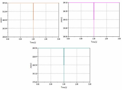
Figure 4. Sensitivity of Df1 detector with failed operating of ARR1, ARR2 and ARR3
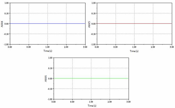
Figure 5. Sensitivity of Df1 detector with normal operating of ARR4, ARR5 and ARR6
The residuals ARR1, ARR2 and ARR3 are sensitive to the failures, it is due to the fact that the Df1 detector appears strongly in these residuals, on the other hand residuals ARR4, ARR5 and ARR6 are null because the detector does not appear in the relations of these residuals it is the normal operating.
Conclusions
The bond graph tool used for modelling and monitoring is very efficient because of the complexity of the phenomena that are produced in the steam condenser as hydraulic and thermal phenomena and the separation between steam and liquid phases.
The Analytical Redundancy Relations are deduced from graphical model of the steam condenser of the distillation column.
The structural junction equations and constitutive element laws for generating these relations are used as the failures indicators.
The algorithm used for researching the optimal case is very efficient.
The simulator of Symbols Software allows the validation and simulation of the model. The technique applied to steam condenser for components monitoring can be extended to detect and locate failures actuators and sensors.
Acknowledgements
Corresponding author would like to thank Prof. Mohammed Mostefai my PhD supervisor and Prof. Mabrouk Khemliche the Head of Automatic Laboratory of Setif –Algeria for performing the present work.
References
1. Raudensky M., Hnizdil M., Hwang J. Y., Lee S. H., Kim S. Y., Influence of the water temperature on the cooling intensity of mist nozzles in continuous casting, Journal of materiali in tehnologije / Materials and Technology, 2012, 3, p. 311-315.
2. Latreche S., Khemliche M., Mostefai M., Modeling and simulation of the distillation column boiler, Asian Journal on Information Technology, 2006, 5(8), p. 823-828.
3. Nan T., Jinjia W., Jiabin F., Experimental and numerical study on the thermal performance of a water/steam cavity receiver, Energies Journal, 2013, 6(3), p. 1198-1216.
4. Ould Bouamama B., Thoma J. U., Cassar J.P., Bond graph modeling of steam condensers, In: IEEE International conference on systems, man, and cybernetic Orlando (USA), 1997, p. 490-494.
5. Cicile J.C., Distillation, Absorption, Généralités sur les colonnes de fractionnement, Technique de l’Ingénieur, Traité de Génie des Procédés, J 2 621, 1999.
6. Thoma J.U., Ould Bouamama B, Modelling and simulation in thermal and chemical engineering. Bond graph approach, Springer - Verlag, Berlin, Germany, 2000.
7. Medjaher K., Samantary A. K., Ould Bouamama B, Bond graph model of a vertical U-tube steam condenser coupled with a heat exchanger, International Journal of Simulation Modelling Practice and Theory, 2009, 17(1), p. 228-239.
8. Khemliche M., Ould Bouamama B., Haffaf H, Sensors placement for diagnosability on bond graph model, Sensors and Actuators Journal, Elsevier A-physical, 2006, 4, p. 92-98.
9. Kozak D., Ivandic Z., Kontajic, P, Determination of the critical pressure for a hot-water pipe with a corrosion defect, Materiali in tehnologije / Materials and Technology, 2010, 6, p. 385-390.
10. Badoud A., Khemliche M., Latreche S, Modeling, simulation and monitoring of nuclear reactor using directed graph and bond graph, Proceedings of World Academy of Science, Engineering and Technology, 2009, 37, p. 199-208.