Impact of wind turbine based on double feed induction generator and FACTS devices on power systems

Labiba ADJOUDJ^1*, Fatiha LAKDJA² and Fatima Zohra GHERBI¹

¹ Engineering Department. Intelligent Control and Electrical Power System Laboratory (ICEPS), Djillali Liabes University, Sidi-Bel-Abbes, 22000, Algeria.

² The Department of Electrical Engineering, Saida University, Engineering Department. Intelligent Control and Electrical Power System Laboratory (ICEPS), Djillali Liabes University, Sidi-Bel-Abbes, 22000, Algeria.

E-mails: ADJOUDJ-l@hotmail.fr; flakdja@yahoo.fr; fzgherbi@gmail.com

^* Corresponding author, phone: +213696757946

Abstract

Integration of wind turbines may have significant impacts on power system operation and generation of electricity from wind power has received considerable attention. This paper analyses the impact of integrating wind generation based on double feed induction generators (DFIG) and Flexible AC Transmission System (FACTS) on the voltage collapse and active losses of network IEEE 30 bus test. Therefore, we must choose among FACTS devices, those with specific applications such as maintaining the voltage at the desired value and the control of power flow, SVC is the most effective in the compensation of reactive as well as maintaining the voltage, and TCSC is the best choice for a proper control of power flow and consequently the reduction of active losses. The simulation results show clearly the effect of wind power plants and FACTS on the grid, voltage stability and power quality of electric power system.

Keywords

Power system; Flexible AC Transmission System; Wind power generation; Voltage stability; power flow; Power System Analysis Toolbox

Introduction

Wind energy is becoming one of the most important renewable energy sources, with the increase in the environmental awareness and the passage of environmental regulations; the environmental constraints are having a significant impact on power systems. Making full use of wind energy to generate electricity cannot only reduce the environmental pollution but also reduce the fuel cost of the power system, which brings the considerable economic benefits. Wind energy is the world’s fastest growing renewable energy source [1].

For analysing the effect of connecting wind farms on the voltage profile and the active losses.

Flexible AC Transmission System (FACTS) controllers are used to enhance the system flexibility and increase system loadability. These controllers are used for enhancing dynamic performance of power system. Different FACTS devices, such as Static Var Compensator (SVC), Thyristor Controlled Series Capacitor (TCSC) are among the most potential controllers for application to power system to achieve better controllability. SVC essentially controls the voltage of a bus in a system. TCSC essentially controls power flow over a line [4].

Power System Analysis Toolbox (PSAT) is a MATLAB toolbox for both electric power system analysis and control. Power flow, continuation power flow, optimal power flow, small signal stability analysis, and time-domain simulation can be applied in PSAT.

The toolbox is also provided with a complete graphical interface and a Simulink based one-line network editor [5]. Advantage is that this tool offers an easy interface to simulate power systems, where most of the components of the system are already modelled. In the tool, there are models for wind turbines, loads, buses, electrical machines, voltage regulators, etc. [6].

The main goal of this paper is to enhance the power flow and resolve the voltage instability with the insertion of wind generation and FACTS devices on power systems.

Material and method

Thyristor-controlled series compensator (TCSC)

TCSC vary the electrical length of the compensated transmission line which enables it to be used to provide fast active power flow regulation.

It also increases the stability margin of the system. The simpler TCSC model exploits the concept of a variable series reactance. The series reactance is adjusted automatically, within limits, to satisfy a specified amount of active power flow through it [7].

The model of the TCSC used in this paper is a variable reactance connected in series with transmission line [8] that is:

(1)

The resulting conductance and susceptance are, respectively:

	(2)
	(3)

where Z_k : Impedance of element k; r_k : Resistance of element k; x_k : Reactance of element k; x_TCSC: Maximum reactance of the TCSC; g_k: Conductance of element k; b_k: Series susceptance of element k; Ω_TCSC: number of lines with TCSCs.

The TCSC (Thyristor-Controlled Series Capacitor) can modify the series capacitive reactance of the transmission line. Figure 1 shows the simplified diagram of TCSC [9].

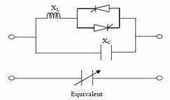
Figure 1. Simple diagram of TCSC

The TCSC is composed of an inductance x_L in series with a thyristor dimmer, all in parallel with a capacitor x_c.

If the thyristors are locked, the TCSC has fixed impedance which corresponds to that of capacitor. If the thyristors are controlled as an electronic switch at full conduction, the TCSC impedance is equal to the equivalent impedance of the capacitor in parallel with the inductance [9]. Figure 2 illustrates the model of TCSC in power flow concept [10].

The TCSC controller is placed between two buses k and m. The equivalent susceptance B_e of the TCSC is function of the firing angle α, the inductance x_L and the capacitor x_c. The susceptance is computed as follow [9]:

(4)

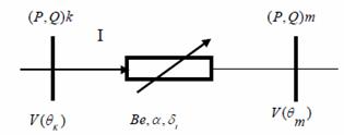
Figure 2. Model of TCSC in a power flow

(P, Q)k are the injected active and reactive powers at bus k, (P,Q)m are the injected active and reactive powers at bus m. The different powers are computed by the following equations [10]:

(5)

where V_k: voltage magnitude at bus n; V_m: voltage magnitude at bus m; B_e : Susceptance; k, m Buses; θ Phase of terminal voltage; δ_t Voltage phase; α Firing angle.  

Static var compensator (SVC)

SVC’s consist of conventional thyristors which have a faster control over the bus voltage and require more sophisticated controllers compared to the mechanical switched conventional devices. SVC’s are shunt connected devices capable of generating or absorbing reactive power. By having a controlled output of capacitive or inductive current, they can maintain voltage stability at the connected bus [11]. SVC devices can be modelled as a variable shunt susceptance [8,12]. Hence, the reactive power injected by the SVC at bus n is:

(6)

where  Q_SVC,n : Reactive power injected by the SVC device at bus n;  b_SVC,n  : Susceptance of the SVC device at bus n; V_n : voltage magnitude at bus n; N_SVC : number of buses with SVCs.

Double feed induction generators (DFIG) model

The overall scheme for a wind farm based on DFIG is depicted in Figure 3. Thus; it is composed by two voltage fed PWM converters in back-to-back configuration. These converters allow the decoupled control of the active and reactive power flow between the DFIG and the AC network by adjusting the switching of the IGBTs.

For this structure, the equations of the double feed induction generator in terms of the d and q axes and neglecting the stator and rotor flux transients can be written as [2,13]:  

For the stator circuit:

	(7)
	(8)

For the rotor circuit:

	(9)
	(10)

where v_ds, v_qs : d and q axes stator voltages; v_dr,v_qr :d and q axes rotor voltages; i_ds,i_qs : d and q axes stator currents; i_dr,i_qr d and q axes rotor currents; R_s, R_r : Stator and rotor resistances; x_s : Stator self-reactance; x_r: Rotor self-reactance; x_m : Mutual reactance; : Rotor speed.

Assuming a lossless converter model, active power of the converter coincides with the rotor active power. The reactive power injected into the grid can be approximated neglecting stator resistance and assuming that the d- axis coincides with the maximum of the stator flux. Therefore, the powers injected in the grid result [14]:

	(11)
	(12)

where  is the grid voltage magnitude.

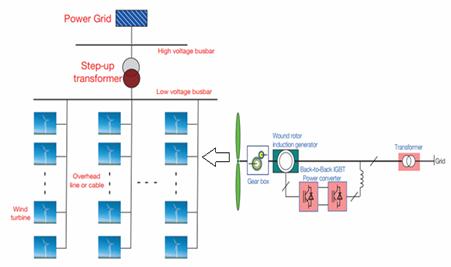
Figure 3. Variable speed wind turbine with doubly fed induction generator

Power flow equations

The current operating condition is defined by the active and reactive power balance at all buses:

	(13)
	(14)

where P_Gn : Total active power production at bus n; P_Dn: Total active power consumption at bus n;  Q_Gn : Total reactive power production at bus n;  Q_Dn : Total reactive power consumption at bus n; P_nm: Active power flow from bus n to bus m as a function of the state variables; Q_nm: Reactive power flow from bus n to bus m as a function of the state variables; N: set of buses; : set of buses connected to bus n.

Transmission lines are modelled by the well-known equivalent p-circuit. The active and reactive power flows from bus n to bus m are [8,12], respectively:

	(15)
	(16)

where: Voltage angle at bus n; : Voltage angle at bus m; V_n,m: Voltage magnitude at bus m, n ;: set of transmission lines; b_pk: shunt susceptance of element k.

Results and discussion

The IEEE 30 Bus Test Case represents a portion of the American Electric Power System (in the Midwestern US) as of December, 1961. The data was kindly provided by Iraj Dabbagchi of AEP and entered in IEEE Common Data Format by Rich Christie at the University of Washington in August 1993[15]. The IEEE 30 bus test system is selected for study to increase the power flow and to get better the voltage profile of the system with 100MVA base, 135 KV base and frequency as 60Hz. The system has 34 transmission lines, 21 load buses, 6 generation buses and 2 fixed capacitors.

System load is kept constant at 283.4MW and 126.2MVAR. The PSAT model for IEEE 30 bus system with base conditions is shown in Figure 4. The following three study cases are addressed here:

§ Case A: impact of SVC and TCSC on system.

§ Case B: impact of wind turbine on system.

§ Case C: impact of wind turbine with FACTS on system.

Figure 4. IEEE 30 bus test system inserted in PSAT

Case A: impact of SVC and TCSC on system

The choice of the optimal location of SVC is based on determination of the bus with the lowest voltage magnitude. The bus is determined by analysing the power flow (Newton Raphson method). Bus 30 is indicated as the critical voltage bus needing Q support.

The TCSC control powers in the transmission lines in order to minimize power losses, the index used in this study for the optimal location of the TCSC, is to determine the most line causes significant losses using the power flow with Newton Raphson method, it is line  between bus 2 and bus 5. The parameters of FACTS devices used in this paper are as follows:

Parameters of TCSC

§ Power, Voltage and Frequency Ratings [MVA, kV, Hz]: [100,135,60];

§ Model type : Xc;

§ Percentage of series compensation [%] : 40;

§ Regulator time constant Tr [s]: 1;

§ Xc_max and Xc_min [p.u. p.u.]: [0.5 -0.5];

§ Proportional and Integral gains Kp and Ki: [5 1];

§ Gain for stabilizing signal Kr [p.u./p.u.]: 10.

Parameters of SVC:

§ Power, Voltage and Frequency Ratings [MVA, kV, Hz]: [100   135   60];

§ Regulator Time Constant Tr [s]: 10;

§ Regulator Gain Kr [p.u./p.u.]: 100;

§ Reference Voltage [p.u.]: 1;

§ B_max and B_min [p.u. p.u.]: [1 -1].

After the optimal location of the SVC was determined to be at bus 30 and TCSC to be between bus 2 and bus 5, Voltages profiles of base case and system with SVC are illustrated in Figure 5. Losses of real power of base case and system with TCSC are shown in Figure 6.

SVC connected to bus 30 injected 5.6878 MVAR to maintain the voltage at the desired value. From the results of voltage profiles without SVC, buses that are relatively far from production units namely bus 24, 25, 26 and 30 have lower voltages relative to the others, this is due to the long distance between the production and consumption. 

Moreover, the installation of the SVC at bus 30 enhances the voltage profile at different bus. The TCSC is adjusted automatically and takes a value of Xc=0.0793 pu between bus 2 and 5. According to the results illustrated in Figure 6, TCSC lowers total losses in the system by17.614 MW to the value 13.0226 MW.

Figure 5. Voltages profiles of test system with and without SVC.

Figure 6. Active Losses of test system with and without TCSC

Table 1. Total generation, losses and slack bus production with and without FACTS

Results	Total generation		Total losses		Slack bus production
	P [MW]	Q[Mvar]	P [MW]	Q[Mvar]	P[MW]	Q[Mvar]
Base case	301.014	172.5027	17.614	46.2427	261.014	-14.3798
with TCSC	296.4226	168.0928	13.0226	41.8328	256.4226	4.0527
With SVC	300.9747	172.3182	17.5747	46.0582	260.9747	-14.836

Case B: impact of wind farm on system

Bus 10 is the most suitable bus (fixed capacitor Bus) and accordingly wind farm of 600 MVA / 69kV capacity comprising of 300 wind turbines which have been connected to this bus by creating another bus (bus no: 31) through a transformer of tap ratio unity.

Wind was modelled after Weibull distribution as proposed by Milano. F (2005) by taking into account the composite nature of wind which included average, ramp, gust, turbulence and low pass filters were used to smooth the wind speed variations[16]. Parameters of DFIG and Wind model are given in Table 2.

The PSAT model for IEEE 30 bus test system with wind turbine is shown in Figure 7, the wind speed and wind power of DFIG are shown in Figure 8 and 9 respectively. The calculation of the power flow is a stage necessary to be able to compare the results. It is performed first for the determination of the initial conditions of the system before the insertion of the power wind.

From Table 3, it is clear that the wind farm lowers total active losses in the system by 17.614 MW to the value 11.8316 MW that is to say a profit of 5.7824 MW and total reactive losses by 46.2426 MVAR to 26.5888 MVAR, a profit of 19.6538 MVAR.

Table 2. DFIG and wind model parameters

Power, Voltage and Frequency Ratings [MVA, kV, Hz]	[600, 69, 60]
Stator Resistance Rs, stator Reactance Xs [p.u, p.u.]	[0.01,  0.10]
Rotor Resistance Rr, Rotor Reactance Xr [p.u, p.u.]	[0.01,  0.08]
Magnetization Reactance Xm [p.u.]	[3.00]
Pitch control gain Kp,  time constant Tp [p.u, s]	[10, 3]
Voltage control gain Kv, Power Control time constant Te [p.u, s]	[10, 0.01]
Number of Pole, gear box ratio [int, -]	[4, 1/89]
Blade length, number  [m, int]	[75.00,  3]
Pmax and Pmin [p.u, p.u.]	[1.00,  0.00]
Qmax and Qmin [p.u, p.u.]	[0.7,  -0.7]
Number of generators	300
Nominal wind speed, air density [m/s, kg/m3]	[15, 1.225]
Filter time constant, sample time [s, s]	[4, 0.1]
Weibull constant C and K	[20, 2]
Ramp constants tsr, ter and Awr [s, s, m/s]	[5, 15, 1]
Gust constants tsg,  teg and Awg [s, s, m/s]	[5, 15, 0]
Turbulence constants h, Z0, Δ f and  n [m, -, Hz, -]	[50, 0.01, 0.2, 50]

The wind farm produced 66,3576MW and 1.0976 MVAR and increase buses that are relatively near from wind production namely bus 3, 4, 5,6,7,8 and 9. Buses 25, 26,27,28,29 and 30 have lower voltages relative to the other.

Table 3. Total generation, losses and slack bus production with and without wind farm.

Results	Total generation		Total losses		Slack bus production
	P [MW]	Q[Mvar]	P [MW]	Q [Mvar]	P[MW]	Q[Mvar]
Base case	301.014	172.5027	17.614	46.2427	261.014	-14.3798
with wind farm	295.2316	152.8488	11.8316	26.5888	188.5556	-3.0583

Figure 7. IEEE 30 bus test system with wind farm inserted in PSAT

Figure 8. Wind speed of DFIG (m/s)

Figure 9. Wind power of DFIG (pu)

Case C: impact of wind farm with FACTS on system

In this part, the effect of connecting wind farm with FACTS. SVC connected to bus 30 produced 6.2983 MVAR to maintain the voltage at the desired value. The installation of the SVC at bus 30 with wind farm enhances the voltage profile at different buses. The TCSC takes a value of Xc=0.7932 pu. From the results, the wind farm at bus 10 and TCSC between bus 2 and bus 5 lowers total losses in the system by17.614 MW to the value 8.506 MW.

Voltages profiles of the base case, the system with wind farm and, finally, the system with wind farm and SVC are illustrated in Figure 10. Losses of real power of base case, system with wind farm and finally system with wind farm and TCSC are shown in Figure 11.

Figure 10. Voltage profiles in different cases

Figure 11. Active losses in different cases

Total energy generated by wind turbines in different cases is shown in Figure 12. The total energy generated and the total energy losed of active and reactive power in different cases, are shown in Figure 13 and Figure 14 respectively.

Figure 12. Generation of wind farm in different cases

Figure 13. Total generation of system in different cases	Figure 14. Total losses of system in different cases

From the results of the simulations, the total generation and losses of system were decreased after the insertion of wind generation and FACTS devices and the proposed approach yields better results.

Conclusions

Simulation was illustrated by the use of one of the most recent software which is software PSAT. This latter was applied without any failure or instability in simulation. Different cases have been tested on IEEE 30 bus test system and presented to show the efficiency of the wind integration and FACTS on power systems. The first part showed the positive contribution of the integration of FACTS devices in the network on voltage profile and power transmitted. The Thyristor controlled series capacitor (TCSC) is one of the most popular FACTS controllers, and this device is the best choice for increasing the line power transfer as well as to enhance the voltage profile of the system. Simulation results show that Static Var Compensator (SVC) generates or absorbs reactive power whose output is adjusted to exchange capacitive or inductive current to maintain or control specific parameters of the electrical power system, typically the bus voltage. The second part was devoted to the integration of wind sources, the application of the proposed approach on IEEE 30 bus test system yields better results, which has concluded that the use of wind farms has significant benefits in reducing the real and reactive power loss and the increase of the voltage profile. The total generation of system and slack bus production were reduced after the insertion of wind farm. Finally, from the results presented in this paper it can conclude that the integration of wind farm with FACTS enhances the power flow and resolve the voltage instability.

References

1. Gonggui C., Jinfu C., Xianzhong D., Power flow and Dynamic optimal power flow including wind farms, sustainable power generation and supply, SUPERGEN 09, 2009, p. 1-6.

2. Munoz J. C., Canizares C. D., comparative stability analysis of DFIG-based wind farm and conventional synchronous generators, IEEE Power System cConference and Exposition (PSCE), 2011, p. 1-7.

3. Awad E. A., Badran  E. A., Youssef F. M. H., Mitigation of Switching Overvoltages due to Energization Procedures in Grid-Connected Offshore Wind Farms, International Journal of Advanced Research in Electrical, Electronics and Instrumentation Engineering, 2014, 3(1), p. 7020- 7028.

4. Somasundaraml P., Muthuselvan N. B., Security constrained optimal power flow with FACTS devices Using modified particle swarm Optimisation, Springer-Verlag Berlin Heidelberg, 2010, 6466, p. 639-646.

5. Milano F., An Open source power system analysis Toolbox, IEEE Transactions on power Systems, 2005, 20(3), p. 1199-1206.

6. Pokhrel B. R., Adhikary B., Study of Wind penetration and its impacts in Kathmandu Valley , IEEE ICSET, 2010, p. 1-5.

7. Sreejith S., Sishaj P. S., Selvan M. P., Power flow analysis incorporating Firing Angle Model Based TCSC, ^5th international conference on industrial and information System ICIIS, 2010, p. 496-501.

8. ZarateMinano R., Conejo A. J., Milano F., OPF-based security redispatching including FACTS devices, IET Gener. Transm. Distrib, 2008, 2(6), p. 821-833.

9. Lakdja F., Ould abdeslam D., Gherbi F. Z., Optimal Location of Thyristor-Controlled Series Compensator for Optimal Power Flows, International review on Modeling and simulations (I.R.E.M.O.S), 2008, 6(2), p. 465-472.

10. Gherbi F. Z., Lakdja F., Berber R., Boudjella H., Dispatching économique au moyen du dispositif FACTS, Acta Electrotehnica, 2010,51(1), p. 51-55.

11. Singh B., Introduction to FACTS Controllers in wind Power Farms a technological review, International Journal of Renewable Energy Research, 2012, 2(2), p. 166-212.

12. Adjoudj L., Lakdja F., Gherbi F. Z., Ould Abdeslam D., Synthesis integrating wind generation and FACTS of network, international  conference on electrical sciences and technologies in maghreb (CISTEM), 2014.

13. Babu B. C., Mohanty K. B., Poongothai C., Wind turbine driven doubly feed induction generator with grid disconnection, in Magnetism, 1963, III G. T. Rado and H. Suhl, Eds. New York: Academic, pp. 271-350.

14. Milano F., Power flow analysis toolbox documentation for PSAT version 2.0.0, 2008.

15. Power Systems Test Case Archive [online], Available at: https://www.ee.washington.edu/research/pstca/pf30/pg_tca30bus.htm.

16. Sasidharan S., Weerakorn O., Singh J. G., Maximisation of instantaneous wind penetration using particle swarm optimisation, international journal of Engineering science and Technology, 2010, 2(5), p. 39-50.